Question: Populations of aphids and ladybugs are modeled
Populations of aphids and ladybugs are modeled by the equations
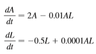
(a) Find the equilibrium solutions and explain their significance.
(b) Find an expression for dL/dA.
(c) The direction field for the differential equation in part (b) is shown. Use it to sketch a phase portrait. What do the phase trajectories have in common?
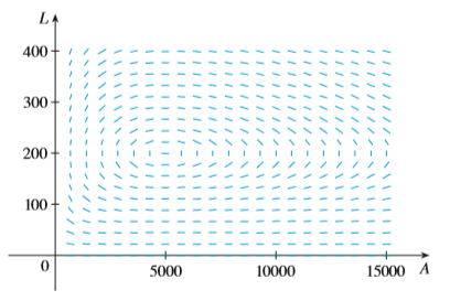
(d) Suppose that at time t = 0 there are 1000 aphids and 200Â ladybugs. Draw the corresponding phase trajectory and use it to describe how both populations change.
(e) Use part (d) to make rough sketches of the aphid and lady bug populations as functions of t. How are the graphs related to each other?
Transcribed Image Text:
dA 2A – 0.01AL dt dL -0.5L + 0.0001AL dt LA 400 300 200 100 5000 10000 15000 A I///- III
> The Pacific halibut fishery has been modeled by the differential equation where y(t) is the biomass (the total mass of the members of the population) in kilograms at time t (measured in years), the carrying capacity is estimated to be M âˆ&#
> Find the radius of convergence and interval of convergence of the series. (r+ 6)" 一1 ー 84
> Suppose that a population grows according to a logistic model with carrying capacity 6000 and k = 0.0015 per year. (a) Write the logistic differential equation for these data. (b) Draw a direction field (either by hand or with a computer algebra system)
> Suppose that a population develops according to the logistic equation where t is measured in weeks. (a) What is the carrying capacity? What is the value of k? (b) A direction field for this equation is shown. Where are the slopes close to 0? Where are th
> A population grows according to the given logistic equation, where t is measured in weeks. (a) What is the carrying capacity? What is the value of k? (b) Write the solution of the equation. (c) What is the population after 10 weeks? dP 0.02P – 0.0004
> A population grows according to the given logistic equation, where t is measured in weeks. (a) What is the carrying capacity? What is the value of k? (b) Write the solution of the equation. (c) What is the population after 10 weeks? dP P 0.04P( 1 dt
> To account for seasonal variation in the logistic differential equation, we could allow k and M to be functions of t: (a) Verify that the substitution z = 1/P transforms this equation into the linear equation (b) Write an expression for the solution of t
> (a) Show that the substitution z = 1/P transforms the logistic differential equation P = kP (1 - P/M) into the linear differential equation (b) Solve the linear differential equation in part (a) and thus obtain an expression for P(t). Compare with Equati
> If we ignore air resistance, we can conclude that heavier objects fall no faster than lighter objects. But if we take air resistance into account, our conclusion changes. Use the expression for the velocity of a falling object in Exercise 35(a) to find d
> An object with mass m is dropped from rest and we assume that the air resistance is proportional to the speed of the object. If s(t) is the distance dropped after t seconds, then the speed is v = s(t) and the acceleration is a = v(t). If t is the acceler
> A tank with a capacity of 400 L is full of a mixture of water and chlorine with a concentration of 0.05 g of chlorine per liter. In order to reduce the concentration of chlorine, fresh water is pumped into the tank at a rate of 4 L/s. The mixture is kept
> In Section 9.3 we looked at mixing problems in which the volume of fluid remained constant and saw that such problems give rise to separable differentiable equations. (See Example 6 in that section.) If the rates of flow into and out of the system are di
> Find the radius of convergence and interval of convergence of the series. (x + 2)" Σ n-2 2" In n
> Two new workers were hired for an assembly line. Jim processed 25 units during the first hour and 45 units during the second hour. Mark processed 35 units during the first hour and 50 units the second hour. Using the model of Exercise 31 and assuming tha
> Let P(t) be the performance level of someone learning a skill as a function of the training time t. The graph of P is called a learning curve. In Exercise 9.1.15 we proposed the differential equation as a reasonable model for learning, where
> In the circuit of Exercise 29, R = 2 V, C − 0.01 F, Q(0) = 0, and E(t) = 10sin 60t. Find the charge and the current at time t. Data from Exercise 29: The figure shows a circuit containing an electromotive force, a capacitor with a cap
> The figure shows a circuit containing an electromotive force, a capacitor with a capacitance of C farads (F), and a resistor with a resistance of R ohms (V). The voltage drop across the capacitor is Q/C, where Q is the charge (in coulombs), so in this ca
> In the circuit shown in Figure 4, a generator supplies a voltage of E(t) = 40 sin 50t volts the inductance is 1 H, the resistance is 20 V, and I(0) = 1 A. (a) Find I(t). (b) Find the current after 0.1 seconds. (c) Use a graphing device to draw the graph
> In the circuit, a battery supplies a constant voltage of 40 V, the inductance is 2 H, the resistance is 10 V, and I(0) = 0. (a) Find I(t). (b) Find the current after 0.1 seconds.
> Solve the second-order equation xyn + 2y’ = 12x2 by making the substitution /
> Use the method of Exercise 23 to solve the differential equation. Data from Exercise 23: A Bernoulli differential equation (named after James Bernoulli) is of the form Observe that, if n = 0 or 1, the Bernoulli equation is linear. For other values of
> Use the method of Exercise 23 to solve the differential equation. Data from Exercise 23: A Bernoulli differential equation (named after James Bernoulli) is of the form Observe that, if n = 0 or 1, the Bernoulli equation is linear. For other values of
> A Bernoulli differential equation (named after James Bernoulli) is of the form Observe that, if n = 0 or 1, the Bernoulli equation is linear. For other values of n, show that the substitution u = y1-n transforms the Bernoulli equation into the linear eq
> Find the radius of convergence and interval of convergence of the series. (-1)" Σ (2n – 1)2" - (x – 1)" n-1
> Solve the differential equation and use a calculator to graph several members of the family of solutions. How does the solution curve change as C varies? ху' — xy' х3 + 2у
> Solve the differential equation and use a calculator to graph several members of the family of solutions. How does the solution curve change as C varies? ху' + 2у— е*
> Solve the initial-value problem. dy + 3x(у — 1) — о, у(0) — 2 dx %3D (x² + 1)
> Solve the initial-value problem. ху' — у + x* sin x, у(п) — 0
> Solve the initial-value problem. ху' + у — x Iп х, у(1) — 0
> Solve the initial-value problem. du — ? + Зи, 1> 0, и(2) — 4 dt
> Solve the initial-value problem. dy + 31'у — сos t, У(т) — 0 dt
> Solve the initial-value problem. x'у + 2ху — In x, у(1) — 2
> Solve the differential equation. dr t In t +r = te' dt
> Solve the differential equation. dy 12 + 3ty = vI + 1², t>0 dt V1 + 1² t > 0
> Find the radius of convergence and interval of convergence of the series. (х — 2)" .2 + 1 n-o n° + 1
> (a) Approximate f by a Taylor polynomial with degree n at the number a. (b) Use Taylor’s Inequality to estimate the accuracy of the approximation / when x lies in the given interval. (c) Check your result in part (b) by graphing / S
> Solve the differential equation. у + 2ху — 1
> Solve the differential equation. ху x>0
> Solve the differential equation. 2ху' + у — 2
> Solve the differential equation. xy' + y = Vx
> Solve the differential equation. 4x'y + x*y' = sin'x
> Solve the differential equation. y' = x - y
> Solve the differential equation. y' - y = e*
> Solve the differential equation. y' + y = 1
> Determine whether the differential equation is linear. dR + t cos R = e dt
> Determine whether the differential equation is linear. du ue' =t + Vi dt
> Find the radius of convergence and interval of convergence of the series. 2n i n!
> In Exercise 10 we modeled populations of aphids and ladybugs with a Lotka-Volterra system. Suppose we modify those equations as follows: (a) In the absence of ladybugs, what does the model predict about the aphids? (b) Find the equilibrium solutions. (c)
> In Example 1 we used Lotka-Volterra equations to model populations of rabbits and wolves. Let’s modify those equations as follows: (a) According to these equations, what happens to the rabbit population in the absence of wolves? (b) Fin
> In Example 1(b) we showed that the rabbit and wolf populations satisfy the differential equation By solving this separable differential equation, show that where C is a constant. It is impossible to solve this equation for Was an explicit function of R (
> Graphs of populations of two species are shown. Use them to sketch the corresponding phase trajectory. y A species 1 1200 1000 800 600 400 species 2 200 10 15
> Graphs of populations of two species are shown. Use them to sketch the corresponding phase trajectory. y species 1 200 species 2 150 - 100 50
> A phase trajectory is shown for populations of rabbits (R) and foxes (d). (a) Describe how each population changes as time goes by. (b) Use your description to make a rough sketch of the graphs of R and F as functions of time. FA 160 1=0 120 80 400
> A phase trajectory is shown for populations of rabbits (R) and foxes (d). (a) Describe how each population changes as time goes by. (b) Use your description to make a rough sketch of the graphs of R and F as functions of time. FA 300 200 100 t=0 400
> Lynx eat snowshoe hares and snowshoe hares eat woody plants like willows. Suppose that, in the absence of hares, the willow population will grow exponentially and the lynx population will decay exponentially. In the absence of lynx and willow, the hare p
> The system of differential equations is a model for the populations of two species. (a) Does the model describe cooperation, or competition, or a predator-prey relationship? (b) Find the equilibrium solutions and explain their significance. dx 0.5x –
> Find the radius of convergence and interval of convergence of the series. n Σ 2"(n² + 1) x" =1
> Each system of differential equations is a model for two species that either compete for the same resources or cooperate for mutual benefit (flowering plants and insect pollinators, for instance). Decide whether each system describes com- petition or coo
> For each predator-prey system, determine which of the variables, x or y, represents the prey population and which represents the predator population. Is the growth of the prey restricted just by the predators or by other factors as well? Do the predators
> Investigate the family of curves defined by the parametric equations x = cos t, y = sin t - sin ct, where c > 0. Start by letting c be a positive integer and see what happens to the shape as c increases. Then explore some of the possibilities that occur
> The curves with equations x = asin nt, y = bcos t are called Lissajous figures. Investigate how these curves vary when a, b, and n vary. (Take n to be a positive integer.)
> Graph several members of the family of curves x = sin t + sin nt, y = cos t + cos nt, where n is a positive integer. What features do the curves have in common? What happens as n increases?
> Graph several members of the family of curves with parametric equations x = t + a cos t, y = t + a sin t, where a > 0. How does the shape change as a increases? For what values of a does the curve have a loop?
> The swallowtail catastrophe curves are defined by the parametric equations x = 2ct - 4t3, y = 2ct2 + 3t4. Graph several of these curves. What features do the curves have in common? How do they change when c increases?
> Investigate the family of curves defined by the parametric equations x = t2, y = t3 - ct. How does the shape change as c increases? Illustrate by graphing several members of the family.
> Suppose that the position of one particle at time t is given by and the position of a second particle is given by (a) Graph the paths of both particles. How many points of intersection are there? (b) Are any of these points of intersection collision poin
> Find the radius of convergence and interval of convergence of the series. (-1)"-1 Σ n5" n-1
> (a) Find parametric equations for the set of all points P as shown in the figure such that |OP|−|AB|. (This curve is called the cissoid of Diocles after the Greek scholar Diocles, who introduced the cissoid as a graphical method for con
> A curve, called a witch of Maria Agnesi, consists of all possible positions of the point P in the figure. Show that parametric equations for this curve can be written as Sketch the curve. х — 2а сot 0 y = 2a sin?e C yA y=2a -- a+
> Compare the curves represented by the parametric equations. How do they differ? (a) x= t, y= t² (с) х — е', у—е " (b) х — сos t, у — sec't
> Compare the curves represented by the parametric equations. How do they differ? (a) x = t°, y= t² (c) x= e , y = e " (b) х — 19, у — 31 21
> Use a graphing calculator or computer to reproduce the picture. yA 3 8 4. 2.
> Use a graphing calculator or computer to reproduce the picture. YA 2- 2
> Find the radius of convergence and interval of convergence of the series. (-1)"4" n-
> (a) Find parametric equations for the ellipse x2/a2 + y2/b2 = 1. (b) Use these parametric equations to graph the ellipse when a = 3 and b = 1, 2, 4, and 8. (c) How does the shape of the ellipse change as b varies?
> Find parametric equations for the path of a particle that moves along the circle x2 + (y - 1)2 = 4 in the manner described. (a) Once around clockwise, starting at (2, 1) (b) Three times around counterclockwise, starting at (2, 1) (c) Halfway around count
> Use a graphing device and the result of Exercise 31(a) to draw the triangle with vertices A(1, 1), B(4, 2), and C(1, 5). Data from Exercise 31: (a) Show that the parametric equations where 0 (b) Find parametric equations to represent the line segment f
> (a) Show that the parametric equations where 0 (b) Find parametric equations to represent the line segment from (22, 7) to (3, 21). x= x, + (x2 – xi)t y = yı + (y2 – yı)t
> Graph the curves y = x3 - 4x and x = y3 - 4y and find their points of intersection correct to one decimal place.
> Match the parametric equations with the graphs labeled I–VI. Give reasons for your choices. (Do not use a graphing device.) (a) x = 1ª – t + 1, y=t² (b) х — ? - 21, у — (c) x = sin 2t, y= sin(t + sin 2i) (d) x = cos 5t, y= sin 2t
> Use the graphs of x = f(t) and y = t(t) to sketch the parametric curve x = f(t), y = t(t). Indicate with arrows the direction in which the curve is traced as t increases. XA 1
> Use the graphs of x = f(t) and y = t(t) to sketch the parametric curve x = f(t), y = t(t). Indicate with arrows the direction in which the curve is traced as t increases. XA 1. -1 1 1
> Use the graphs of x = f(t) and y = t(t) to sketch the parametric curve x = f(t), y = t(t). Indicate with arrows the direction in which the curve is traced as t increases. XA
> Find the radius of convergence and interval of convergence of the series. E 2"n?x" n=1
> Match the graphs of the parametric equations x = f(t) and y = t(t) in (a)–(d) with the parametric curves labeled I–IV. Give reasons for your choices. (a) I 2 1 2 x (b) II XA YA 2. y 2- 2 x (c) III y 1 2 x (d) I
> Describe the motion of a particle with position sx, yd as t varies in the given interval. x = sin 1, y = cos?t, -27 < t< 2m
> Describe the motion of a particle with position sx, yd as t varies in the given interval. x = 5 sin t, y = 2 cos t, -T<I< 5T
> Describe the motion of a particle with position sx, yd as t varies in the given interval. x = 2 + sin t, y=1 + 3 cos t, T/2<1<27
> Describe the motion of a particle with position sx, yd as t varies in the given interval. x = 5 + 2 cos T t, y=3 + 2 sin mt, 1<t<2
> (a) Eliminate the parameter to find a Cartesian equation of the curve. (b) Sketch the curve and indicate with an arrow the direction in which the curve is traced as the parameter increases. х — tan'o, у — sec 0, —п/2 <0 < п/2
> (a) Eliminate the parameter to find a Cartesian equation of the curve. (b) Sketch the curve and indicate with an arrow the direction in which the curve is traced as the parameter increases. x = sinh t, y= cosh t
> (a) Eliminate the parameter to find a Cartesian equation of the curve. (b) Sketch the curve and indicate with an arrow the direction in which the curve is traced as the parameter increases. x = /i + 1, y= vi - 1
> (a) Eliminate the parameter to find a Cartesian equation of the curve. (b) Sketch the curve and indicate with an arrow the direction in which the curve is traced as the parameter increases. x = t, y= In t
> (a) Eliminate the parameter to find a Cartesian equation of the curve. (b) Sketch the curve and indicate with an arrow the direction in which the curve is traced as the parameter increases. 21 x = e', y
> Find the radius of convergence and interval of convergence of the series. Σ n*4"
> (a) Eliminate the parameter to find a Cartesian equation of the curve. (b) Sketch the curve and indicate with an arrow the direction in which the curve is traced as the parameter increases. х — sin t, у - csc i, 0 <1< п/2
> (a) Eliminate the parameter to find a Cartesian equation of the curve. (b) Sketch the curve and indicate with an arrow the direction in which the curve is traced as the parameter increases. x =} cos 0, y = 2 sin 0, 0< 0 <
> (a) Eliminate the parameter to find a Cartesian equation of the curve. (b) Sketch the curve and indicate with an arrow the direction in which the curve is traced as the parameter increases. х — sin 0, y — сos s0, -<0 < T
> (a) Sketch the curve by using the parametric equations to plot points. Indicate with an arrow the direction in which the curve is traced as t increases. (b) Eliminate the parameter to find a Cartesian equation of the curve. x = t', y = t .2 3. х
> (a) Sketch the curve by using the parametric equations to plot points. Indicate with an arrow the direction in which the curve is traced as t increases. (b) Eliminate the parameter to find a Cartesian equation of the curve. x = /i, y=1 – t Vi,