Question: Read the box “The Demand for Economics
Read the box “The Demand for Economics Journals†in Section 8.3. Discuss the internal and external validity of the estimated effect of price per citation on subscriptions.
Data from Section 8.3:
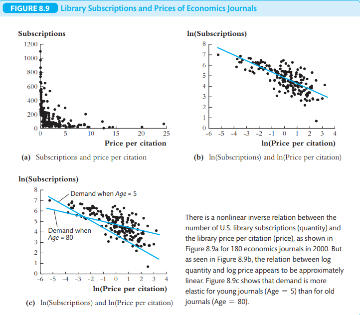
Professional economists follow the most recent research in their areas of specialization. Most research in economics first appears in economics journals, so economists—or their libraries—subscribe to economics journals.
How elastic is the demand by libraries for economics journals? To find out, we analyzed the relationship between the number of subscriptions to a journal at U.S. libraries (Yi) and the journal’s library subscription price using data for the year 2000 for 180 economics journals. Because the product of a journal is the ideas it contains, its price is logically measured not in dollars per year or dollars per page but instead in dollars per idea. Although we cannot measure “ideas†directly, a good indirect measure is the number of times that articles in a journal are subsequently cited by other researchers.
Accordingly, we measure price as the “price per citation†in the journal. The price range is enormous, from 1/2¢ per citation (the American Economic Review) to 20¢ per citation or more. Some journals are expensive per citation because they have few citations and others because their library subscription price per year is very high. In 2017, a library print subscription to the Journal of Econometrics cost $5363, compared to only $940 for a bundled subscription to all eight journals published by the American Economic Association, including the American Economic Review! Because we are interested in estimating elasticities, we use a log-log specification (Key Concept 8.2). The scatterplots in Figures 8.9a and 8.9b provide empirical support for this transformation.
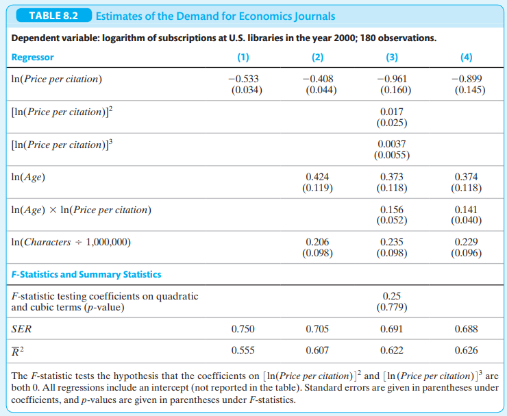
Because some of the oldest and most prestigious journals are the cheapest per citation, a regression of log quantity against log price could have omitted variable bias. Our regressions therefore include two control variables: the logarithm of age and the logarithm of the number of characters per year in the journal. The regression results are summarized in Table 8.2.
Those results yield the following conclusions (see if you can find the basis for these conclusions in the table!):
1. Demand is less elastic for older than for newer journals.
2. The evidence supports a linear, rather than a cubic, function of log price.
3. Demand is greater for journals with more characters, holding price and age constant.
So what is the elasticity of demand for economics journals? It depends on the age of the journal. Demand curves for an 80-year-old journal and a 5-year-old upstart are superimposed on the scatterplot in Figure 8.9c; the older journal’s demand elasticity is -0.28 (SE = 0.06), while the younger journal’s is -0.67 (SE = 0.08).
This demand is very inelastic: Demand is very insensitive to price, especially for older journals. For libraries, having the most recent research on hand is a necessity, not a luxury. By way of comparison, experts estimate the demand elasticity for cigarettes to be in the range of -0.3 to -0.5. Economics journals are, it seems, as addictive as cigarettes but a lot better for your health!
> Consider the regression model with heterogeneous regression coefficients Yi = 0 + 1iXi + vi, where (vi, Xi, 1i) are i.i.d. random variables with 1 = E (1i). a. Show that the model can be written as Yi = 0 + 1Xi + ui, where ui = (1i - 1) Xi + vi.
> How would you calculate the small class treatment effect from the results in Table 13.1? Can you distinguish this treatment effect from the aide treatment effect? How would you have to change the program to correctly estimate both effects? Data from Tab
> Y is distributed N (10, 100) and you want to calculate Pr (Y
> A researcher is interested in the effect of more secure property rights on income across countries. He collects recent data from 60 countries and runs the OLS regression Yi = 0 + 1Xi + ui, where Yi is a country’s GDP per capita and Xi is an index takin
> Consider a product market with a supply function Qsi = 0 + 1Pi + usi, a demand function Qdi = 0 + udi, and a market equilibrium condition Qsi = Qdi, where usi and udi are mutually independent i.i.d. random variables, both with a mean of 0. a. Show tha
> A classmate has developed an IV regression model with one regressor, Xi, and two instruments, Z1i and Z2i. She has a strong theoretical basis as to why corr (Z1i, ui) = 0, namely that Z1i is the result of a random lottery. Preliminary work, however, show
> Suppose a researcher is considering developing an IV regression model with one regressor, Xi, and one instrument, Zi. If she has a sample of n = 113, what range must the correlation coefficient be between Xi and Zi in order for Zi to be considered a stro
> Consider the IV regression model Yi = 0 + 1Xi + 2Wi + ui, where Xi is correlated with ui and Zi is an instrument. Suppose that the first three assumptions in key concept are satisfied. Which IV assumption is not satisfied when a. Zi is independent of
> Consider TSLS estimation of the effect of a single included endogenous variable, Xi, on Yi using one binary instrument, Zi, which takes values of either 0 or 1. Noting that show that the Wald estimator can be derived from the TSLS estimator in this circu
> A classmate is interested in estimating the variance of the error term in Equation (12.1). a. Suppose she uses the estimator from the second-stage regression of where X^i is the fitted value from the first-stage regression. Is this estimator consistent?
> Consider the regression model with a single regressor: Yi = 0 + 1Xi + ui. Suppose the least squares assumptions in Key Concept 4.3 are satisfied. a. Show that Xi is a valid instrument. That is, show that Zi = Xi. b. Show that the IV regression assumpti
> Two classmates are comparing their answers to an assignment. One classmate has specified an instrumental variable regression model Yi = 0 + 1Xi + 2Wi + ui, using Zi as an instrument. The other student has specified the same model, but has omitted Wi.
> This question refers to the panel data IV regressions summarized in Table. a. Suppose the federal government is considering a new tax on cigarettes that is estimated to increase the retail price by $0.25 per pack. If the current price per pack is $6.75,
> Suppose Yi, I = 1, 2, …, n is i.i.d. random variables, each distributed N (20, 4). a. Compute Pr (19.6
> Use the estimated linear probability model shown in column (1) of Table 11.2 to answer the following: a. Two applicants, one self-employed and one in salaried employment, apply for a mortgage. They have the same values for all the regressors other than e
> Consider the linear probability model Yi = 0 + 1Xi + ui, and assume that E (ui | Xi) = 0. a. Show that Pr (Yi = 1 | Xi) = 0 + 1Xi. b. Show that var (ui | Xi) = (0 + 1Xi) [1 – (0 + 1Xi)]. c. Is ui heteroskedastic? Explain. d. Derive the likelih
> Repeat Exercise 11.6 using the logit model in Equation (11.10). Are the logit and probit results similar? Explain. Data from Equation 11.10: Data from Exercise 11.6: Use the estimated probit model in Equation (11.8) to answer the following questions: a
> Use the estimated probit model in Equation (11.8) to answer the following questions: a. A black mortgage applicant has a P/I ratio of 0.35. What is the probability that his application will be denied? b. Suppose the applicant reduced this ratio to 0.30.
> Seven hundred income-earning individuals from a district were randomly selected and asked whether they are government employees (Govi = 1) or not (Govi = 0); data were also collected on their gender (Malei = 1 if male and = 0 if female) and their years o
> Seven hundred income-earning individuals from a district were randomly selected and asked whether they are government employees (Govi = 1) or not (Govi = 0); data were also collected on their gender (Malei = 1 if male and = 0 if female) and their years o
> Seven hundred income-earning individuals from a district were randomly selected and asked whether they are government employees (Govi = 1) or not (Govi = 0); data were also collected on their gender (Malei = 1 if male and = 0 if female) and their years o
> Seven hundred income-earning individuals from a district were randomly selected and asked whether they are government employees (Govi = 1) or not (Govi = 0); data were also collected on their gender (Malei = 1 if male and = 0 if female) and their years o
> State which model you would use for: a. A study explaining the number of hours a person spends working in a factory during one week. b. A study explaining the level of satisfaction (0 through 5) a person gains from their job. c. A study of consumers’ cho
> Suppose a random variable Y has the following probability distribution: Pr (Y = 1) = p, Pr (Y = 2) = q, and Pr (Y = 3) = 1 - p - q. A random sample of size n is drawn from this distribution, and the random variables are denoted Y1, Y2, ……, Yn. a. Derive
> In a population, Y = 50 and 2Y = 21. Use the central limit theorem to answer the following questions: a. In a random sample of size n = 50, find Pr (Y 49). c. In a random sample of size n = 45, find Pr (50.5
> Seven hundred income-earning individuals from a district were randomly selected and asked whether they are government employees (Govi = 1) or not (Govi = 0); data were also collected on their gender (Malei = 1 if male and = 0 if female) and their years o
> a. In the fixed effects regression model, are the fixed entity effects, ai, consistently estimated as with T fixed? b. If n is large (say, n = 2000) but T is small (say, T = 4), do you think that the estimated values of i are approxima
> Consider observations (Yit, Xit) from the linear panel data model Yit = Xit1 + i + it + uit, where t = 1, ……, T; i = 1, ……, n; and i + it is an unobserved entity-specific time trend. How would you estimate 1?
> Suppose a researcher believes that the occurrence of natural disasters such as earthquakes leads to increased activity in the construction industry. He decides to collect province-level data on employment in the construction industry of an earthquake-pro
> Do the fixed effects regression assumptions imply that cov (v∼it, v∼is) = 0 for t ≠s in Equation (10.28)? Explain. Data from Equation 10.28:
> Consider the model with a single regressor. This model also can be written as Yit = 0 + 1X1, it + 2B2t + + TBTt + 2D2i ++ nDni + uit, where B2t = 1 if t = 2 and 0 otherwise, D2i = 1 if i = 2 and 0 otherwise, and so forth. How are the coefficien
> Using the regression in Equation (10.11), what are the slope and intercept for a. Entity 1 in time period 1? b. Entity 1 in time period 3? c. Entity 3 in time period 1? d. Entity 3 in time period 3? Data from Equation 1011:
> Section 9.2 gave a list of five potential threats to the internal validity of a regression study. Apply that list to the empirical analysis and thereby draw conclusions about its internal validity. Data from Section 9.2: 1. Omitted Variable Bias 2. Meas
> Consider the binary variable version of the fixed effects model in Equation except with an additional regressor, D1i; that is, let a. Suppose that n = 3. Show that the binary regressors and the “constant” regressor are
> Let ^1DM denote the entity-demeaned estimator given in Equation (10.22), and let ^BA1 denote the “before and after” estimator without an intercept, so that Show that, if Data from E
> X is a Bernoulli random variable with Pr (X = 1) = 0.90; Y is distributed N (0, 4); W is distributed N (0, 16); and X, Y, and W are independent. Let S = XY + (1 – X) W. (That is, S = Y when X = 1, and S = W when X = 0.) a. Show that E(Y2) = 4 and E(W2) =
> A researcher wants to estimate the determinants of annual earnings—age, gender, schooling, union status, occupation, and sector of employment. He has been told that if he collects panel data on a large number of randomly chosen individuals over time, he
> This exercise refers to the drunk driving panel data regression summarized in Table 10.1. a. New Jersey has a population of 8.85 million people. Suppose New Jersey increased the tax on a case of beer by $2 (in 1988 dollars). Use the results in column (5)
> Consider the linear regression of TestScore on Income shown in Figure 8.2 and the nonlinear regression in Equation (8.18). Would either of these regressions provide a reliable estimate of the causal effect of income on test scores? Would either of these
> Would the regression in Equation (4.9) in chapter 4 be useful for predicting test scores in a school district in Massachusetts? Why or why not? Data from Equation 4.9:
> Are the following statements true or false? Explain your answer. a. “An ordinary least squares regression of Y onto X will not be internally valid if Y is correlated with the error term.” b. “If the error term exhibits heteroskedasticity, then the estima
> Suppose that n = 50 i.i.d. observations for (Yi, Xi) yield the following regression results: Y^ = 49.2 + 73.9X, SER = 13.4, R2 = 0.78. Another researcher is interested in the same regression, but he makes an error when he enters the data into his regress
> The demand for a commodity is given by Q = 0 + 1P + u, where Q denotes quantity, P denotes price, and u denotes factors other than price that determine demand. Supply for the commodity is given by Q = 0 + 1P + v, where v denotes factors other than pr
> Using the regressions shown in columns (2) of Table 9.3, and column (2) of Table 9.2, construct a table like Table 9.3 and compare the estimated effects of a 10 percentage point increase in the students eligible for free lunch on test scores in Californi
> Labor economists studying the determinants of women’s earnings discovered a puzzling empirical result. Using randomly selected employed women, they regressed earnings on the women’s number of children and a set of control variables (age, education, occup
> Consider the one-variable regression model Yi = 0 + 1Xi + ui, and suppose it satisfies the least squares assumptions. Suppose Yi is measured with error, so the data are Y∼i = Yi + wi, where wi is the measurement error, which is i.i.d. and independent o
> Compute the following probabilities: a. If Y is distributed t12, find Pr (Y
> Assume that the regression model Yi = 0 + 1Xi + ui satisfies the least squares assumptions. You and a friend collect a random sample of 300 observations on Y and X. a. Your friend reports that he inadvertently scrambled the X observations for 20% of th
> Consider the one-variable regression model Yi = 0 + 1Xi + ui, and suppose it satisfies the least squares assumptions in Key Concept 4.3. The regressor Xi is missing, but data on a related variable, Zi, are available, and the value of Xi is estimated us
> Read the box “The Effect of Ageing on Healthcare Expenditures: A Red Herring?” in Section 8.3. Discuss the internal and external validity as a causal effect of the relationship between age and healthcare expenditures,
> Suppose that you have just read a careful statistical study of the effect of improved health of children on their test scores at school. Using data from a project in a West African district in 2000, the study concluded that students who received multivit
> Explain how you would use approach 2 to calculate the confidence interval discussed below Equation (8.8). Data from Equation 8.8:
> X is a continuous variable that takes on values between 5 and 100. Z is a binary variable. Sketch the following regression functions (with values of X between 5 and 100 on the horizontal axis and values of Y^ on the vertical axis): a. Y^ = 2.0 + 3.0 * ln
> This problem is inspired by a study of the gender gap in earnings in top corporate jobs (Bertrand and Hallock, 2001). The study compares total compensation among top executives in a large set of U.S. public corporations in the 1990s. (Each year these pub
> Refer to Table 8.3. a. A researcher suspects that the effect of %Eligible for subsidized lunch has a nonlinear effect on test scores? In particular, he conjectures that increases in this variable from 10% to 20% have little effect on test scores but that
> Read the box “The Demand for Economics Journals” in Section 8.3. a. The box reaches three conclusions. Looking at the results in the table, what is the basis for each of these conclusions? b. Using the results in regre
> Compute the following probabilities: a. If Y is distributed X23, find Pr (Y
> Read the box “The Effect of Ageing on Healthcare Expenditures: A Red Herring?” a. Consider a male aged 60 years. Use the results from column (1) of Table 8.1 and the method in Key Concept 8.1 to estimate the expected c
> After reading this chapter’s analysis of test scores and class size, an educator comments, “In my experience, student performance depends on class size, but not in the way your regressions say. Rather, students do well when class size is less than 20 stu
> Suppose a researcher collects data on houses that have sold in a particular neighbourhood over the past year and obtains the regression results in the following table. a. Using the results in column (1), what is the expected change in price of building a
> The discussion following Equation (8.28) interprets the coefficient on interacted binary variables using the conditional mean zero assumption. This exercise shows that this interpretation also applies under conditional mean independence. Consider the hyp
> Derive the expressions for the elasticities for the linear and log-log models.
> Consider the regression model Yi = 0 + 1X1i + 2X2i + 31X(i * X2i) + ui. Show that; a. ∆Y>∆X1 = 1 + 3X2 (effect of change in X1, holding X2 constant). b. ∆Y>∆X2 = 2 + 3X1 (effect of change in X2, holding X1 constant). c. If X1 changes by ∆X1 and
> Sales in a company are $243 million in 2018 and increase to $250 million in 2019. a. Compute the percentage increase in sales, using the usual formula 100 * (Sales2019 - Sales2018)/ Sales2013. Compare this value to the approximation 100 * [ln (Sales2019)
> Consider the regression model Yi = 0 + 1X1i + 2X2i + ui. Transform the regression so that you can use a t-statistic to test a. 1 = 2. b. 1 + 22 = 0. c. 1 + 2 = 1. (Hint: You must redefine the dependent variable in the regression.)
> Referring to the Table: a. Construct the R2 for each of the regressions. b. Show how to construct the homoskedasticity-only F-statistic for testing 4 = 5 = 6 = 0 in the regression shown in column (3).
> Reported the following regression (where standard errors have been added): a. Is the coefficient on BDR statistically significantly different from zero? b. Typically, four-bedroom houses sell for more than three-bedroom houses. Is this consistent with yo
> Compute the following probabilities: a. If Y is distributed N (4, 9), find Pr (Y 2). c. If Y is distributed N (1, 4), find Pr (2
> Let Y denote the number of “heads” that occur when two coins are tossed. Assume the probability of a heads is 0.4 on either coin. a. Derive the probability distribution of Y. b. Derive the mean and variance of Y.
> This information has been taken from the company´s books as at 31 December 20X1, but the information below has not been allowed for. (a) Inventory at 31 December 20X1 is €20,000. (b) Plant and machinery is to be depreciated
> The information has been taken from the company´s books as at 31 December 20X1, but the following has not been allowed for: (a) Inventory at the end of the year is €25,000. (b) Audit fees owing amounted to €
> Explain the various advantages and disadvantages of moving to a corporate form of business instead of operating as a partnership.
> Explain the various possible advantages that a number of sole traders might obtain by joining together as a partnership.
> Set out in Figure 16.9 is summarized balance sheets and income statements for F Co. for 20X1 and 20X2. You are required to: (a) prepare a table of ratios, covering all aspects of interpretation as far as the infor- mation allows, for each of the two year
> The details in Figure 16.8 relate to D Co. Using that information and appropriate ratios, prepare a financial report on the company. The opening inventory value figures were €135,000 20X1 actual and €210,000 20X2 budget.
> ‘Financial ratios are only as good as the accounting information from which they are calculated’. Discuss.
> The stated accounting policy treatment for foreign currency translation for SKF, a Swedish company, before it adopted IFRS was as follows: Translation of foreign financial statements The current rate method is used for translating the income statements a
> ‘The variety of possible methods of foreign currency translation, and the different ways of treating gains arising, show that adequate harmonisation for international comparison purposes is a long way away’. Discuss.
> (a) How would you define goodwill? (b) Three possible accounting treatments of goodwill are: (i) retain goodwill as an asset to be amortised over its estimated useful life; (ii) retain goodwill as an asset indefinitely, subjecting it to annual impairment
> The balance sheets of A and B as at 31 December 20X7 are as shown in Figure 14.8. In addition: (a) A had acquired 37,500 shares in B in 20X3 when there was a debit balance on the reserves of €3,000. (b) B purchases goods from A, providin
> Repeat Exercise 13.3, but now assume that non-current assets originally costing €30,000, with accumulated depreciation of €12,000, were sold for €11,000 during the year ended 31 December 20X2.
> If at all possible, compare your answer to Exercise 1.5 with the answers of students from different national backgrounds. Try to explore likely causes of any major differences that emerge, in terms of legal, economic and cultural environments.
> The balance sheet of Dot Co. for the year ended 31 December 20X2, together with comparative figures for the previous year, is shown in Figure 13.7 (all figures €000). You are informed that there were no sales of non-current assets durin
> Explain the concept of a ‘temporary difference’ in the context of IASB rules. Why is it thought necessary to account for deferred tax on these differences?
> In Activity 12.A, the balance on the deferred tax liability account is growing every year over the five-year period and, if tax conditions remain stable and annual investment continues to rise, then it will continue to grow. Could it be argued that, beca
> How might a company seek to raise extra finance in ways other than issuing new debt or equity securities?
> Distinguish between debt capital and equity capital and suggest which is likely to be favored by a company raising finance in a high-taxation environment.
> What uses of the word ‘reserve’ might be found in practice in various parts of the world?
> What is the definition of a fixed (or non-current) asset? Why is this difficult to use in the context of investments and why does that matter?
> What is meant by ‘lower of cost and net realizable value’? What difficulties exist in the application of this measurement basis?
> A firm buys and sells a single commodity. During a particular accounting period it makes a number of purchases of the commodity at different prices. Explain how assumptions made regarding which units were sold will affect the firm’s reported profit for t
> R and A are brothers. Recently, their aunt died leaving them €1,000 each. Initially, they intended setting up in partnership selling pils and lager. However, R felt that there was no future in the lager market, whereas A expected that lager sales would b
> In the context of your own national background, rank the seven ‘external’ user groups suggested in the text (i.e. omitting managers), in order of the priority that you think should be given to their needs. Explain your reasons.
> Using the information contained in Exercise 10.3 above, calculate the value of the year-end inventories using FIFO and LIFO. Also, prepare profit and loss accounts showing the gross profit under each of the valuation methods for all three years.
> Outline three different depreciation methods and appraise them in the context of the definition and objectives of depreciation.
> The payments set out in Table 9.8 have been made during the year in relation to a non-current asset bought at the beginning of the year. What cost figure should be used as the basis for the depreciation charge for the year and why?
> Provide in your own words: (a) an explanation of what depreciation is; (b) an explanation of the net book value (NBV) of a partially depreciated non-current asset.
> A company borrows money at 10 per cent interest in order to finance the building of a new factory. Suggest arguments for and against the proposition that the interest costs should be capitalized and regarded as part of the ‘cost’ of the factory. Which se
> On 21 December 20X7, your client paid €10,000 for an advertising campaign. The advertisements will be heard on local radio stations between 1 January and 31 January 20X8. Your client believes that, as a result, sales will increase by 60 per cent in 20X8
> Are depreciation expenses either too subjective or too arbitrary to provide useful information?