Question: Several applications in this and previous chapters
Several applications in this and previous chapters have examined the returns to education in panel data sets. Specifically, we applied Hausman and Taylor’s approach in Examples 11.17 and 11.18. Example 11.18 used Cornwell and Rupert’s data for the analysis. Koop and Tobias’s (2004) study that we used in Chapters 3 and 5 provides yet another application that we can use to continue this analysis. The data may be downloaded from the Journal of Applied Econometrics data archive at http://qed.econ.queensu.ca/jae/2004-vl9.7/koop-tobias/. The data file is in two parts. The first file contains the full panel of 17,919 observations on variables:
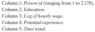
Columns 2 through 5 contain time-varying variables. The second part of the data set contains time-invariant variables for the 2,178 households. These are:

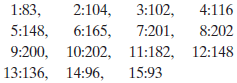
To create the data set for this exercise, it is necessary to merge these two data files. The ith observation in the second file will be replicated Ti times for the set of Ti observations in the first file. The person id variable indicates which rows must contain the data from the second file. (How this preparation is carried out will vary from one computer package to another.) The panel is quite unbalanced; the number of observations by group size is:
Value of Ti
a. Using these data, fit fixed and random effects models for log wage and examine the result for the return to education.
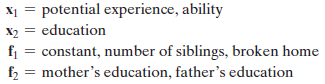
b. For a Hausman–Taylor specification, consider the following:
Based on this specification, what is the estimated return to education? (Note: you may need the average value of 1/Ti for your calculations. This is 0.1854.)
c. It might seem natural to include ability with education in x2. What becomes of the Hausman and Taylor estimator if you do so?
d. Using a different specification, compute an estimate of the return to education using the instrumental variables method.
e. Compare your results in parts b and d to the results in Examples 11.17 and 11.18. The estimated return to education is surprisingly stable.
> Now suppose that the disturbances are not normally distributed, although / is still known. Show that the limiting distribution of the previous statistic is (1/J) times a chi-squared variable with J degrees of freedom. (Hint: The denominator converges t
> This and the next two exercises are based on the test statistic usually used to test a set of J linear restrictions in the generalized regression model, where  is the GLS estimator. Show that if / is known, if the disturbances are nor
> The following table presents a hypothetical panel of data: a. Estimate the group wise heteroscedastic model of section 9.7.2. Include an estimate of the asymptotic variance of the slope estimator. Use a two-step procedure, basing the FGLS estimator at
> The model satisfies the group wise heteroscedastic regression model of section 9.7.2 All variables have zero means. The following sample second-moment matrix is obtained from a sample of 20 observations: a. compute the two separate OLS estimates of &
> Suppose that in the group wise heteroscedasticity model of section 9.7.2, Xi is the same for all i. What is the generalized least squares estimator of ? How would you compute the estimator if it were necessary to estimate 2i?
> Two samples of 50 observations each produce the following moment matrices. (In each case, X is a constant and one variable.) a. compute the least squares regression coefficients and the residual variances s2 for each data set. compute the R2 s for each
> For the model in Exercise 9, suppose that is normally distributed, with mean zero and variance 2[1 + (x)2]. Show that 2 and 2 can be consistently estimated by a regression of the least squares residuals on a constant and x2. Is this estimator efficie
> To continue the analysis in Application 5, consider a nonparametric regression of G/Pop on the price. Using the nonparametric estimation method in Section 7.5, fit the nonparametric estimator using a range of bandwidth values to explore the effect of ban
> For the model in Exercise 9, what is the probability limit of Note that s2 is the least squares estimator of the residual variance. It is also n times the conventional estimator of the variance of the OLS estimator, How does this equation compare with
> What is the covariance matrix, of the GLS estimator and the difference between it and the OLs estimator, The result plays a pivotal role in the development of specification tests in Hausman (1978).
> Prove that in the control function estimator in (8-16), you can use the predictions, z'p, instead of the residuals to obtain the same results apart from the sign on the control function itself, which will be reversed.
> Prove that the control function approach in (8-16) produces the same estimates as 2SLS.
> This is easy to show. In the expression for , if the kth Colum n in X is one of the columns in Z, say the lth, then the kth column in (Z'Z)-1Z'X will be the lth column of an L * L identity matrix. This result means that the kth column in = Z (Z'Z)-1Z
> Consider the linear model, Let z be an exogenous, relevant instrumental variable for this model. Assume, as well, that z is binary—it takes only values 1 and 0. Show the algebraic forms of the LS estimator and the IV estimator for both
> At the end of section 8.7, it is suggested that the OLs estimator could have a smaller mean squared error than the 2sLs estimator. Using (8-4), the results of Exercise 1, and Theorem 8.1, show that the result will be true if How can you verify that thi
> Derive the results in (8-32a) and (8-32b) for the measurement error model. Note the hint in Footnote 4 in section 8.5.1 that suggests you use result (A-66) when you need to invert
> For the measurement error model in (8-26) and (8-27), prove that when only x is measured with error, the squared correlation between y and x is less than that between y* and x*. (Note the assumption that y* = y.) Does the same hold true if y* is also mea
> In the discussion of the instrumental variable estimator, we showed that the least squares estimator, bLs, is biased and inconsistent. Nonetheless, bLs does estimate something—plim Derive the asymptotic covariance matrix of bLs and sh
> In Application 1 in chapter 3 and Application 1 in chapter 5, we examined Koop and Tobias’s data on wages, education, ability, and so on. We continue the analysis here. (The source, location and configuration of the data are given in th
> Verify the following differential equation, which applies to the Box–cox transformation: Show that the limiting sequence for  = 0 is These results can be used to great advantage in deriving the actual second derivatives
> Describe how to obtain nonlinear least squares estimates of the parameters of the model y = ax+ .
> Dummy variable for one observation. Suppose the data set consists of n observations, (yn, Xn) and an additional observation, The full data set contains a dummy variable, d, that equals zero save for one (the last) observation. Then, the full data set is
> Reverse regression continued. suppose that the model in Exercise 3 is extended to y = x* + d + , x = x* + u. For convenience, we drop the constant term. Assume that x*, e, and u are independent normall
> Estimate the parameters of the model in Example 10.4 using two-stage least squares. Obtain the residuals from the two equations. Do these residuals appear to be white noise series? Based on your findings, what do you conclude about the specification of t
> Carry out an ADF test for a unit root in the rate of inflation using the subset of the data in Appendix Table F5.2 since 1974.1. (This is the first quarter after the oil shock of 1973.)
> Using the macroeconomic data in Appendix Table F5.2, estimate by least squares the parameters of the model where ct is the log of real consumption and yt is the log of real disposable income. a. Use the Breusch and Pagan LM test to examine the residuals
> (This exercise requires appropriate computer software. The computations required can be done with RATS, EViews, Stata, LIMDEP, and a variety of other software using only preprogrammed procedures.) Quarterly data on the consumer price index for 1950.1 to
> Data for fitting an improved Phillips curve model can be obtained from many sources, including the Bureau of Economic Analysis’s (BEA) own Web site, www. economagic.com, and so on. Obtain the necessary data and expand the model of Example 20.3. Does addi
> The data used to fit the expectations augmented Phillips curve in Example 20.3 are given in Appendix Table F5.2. Using these data, reestimate the model given in the example. Carry out a formal test for first-order autocorrelation using the LM statistic.
> The application in chapter 3 used 15 of the 17,919 observations in Koop and Tobias’s (2004) study of the relationship between wages and education, ability, and family characteristics. (see Appendix Table F3.2.) We will use the full data set for this exer
> Stochastic Frontier Model. section 10.3.1 presents estimates of a cobb–Douglas cost function using Nerlove’s 1955 data on the U.s. electric power industry. christensen and Greene’s 1976 update of this study used 1970 data for this industry. The christens
> Continuing the analysis of the previous application, note that these data conform precisely to the description of corner solutions in section 19.3.4. The dependent variable is not censored in the fashion usually assumed for a tobit model. To investigate
> The Mroz (1975) data used in Example 19.10 (see Appendix Table F5.1) also describe a setting in which the tobit model has been frequently applied. The sample contains 753 observations on labor market outcomes for married women, including the following va
> We examined Ray Fair’s famous analysis (Journal of Political Economy, 1978) of a Psychology Today survey on extramarital affairs in Example 18.18 using a Poisson regression model. Although the dependent variable used in that study was a count, Fair (1978
> Appendix Table F18.3 contains data on ship accidents reported in McCullagh and Nelder (1983). The data set contains 40 observations on the number of incidents of wave damage for oceangoing ships. Regressors include aggregate months of service, and three
> The GSOEP data are an unbalanced panel, with 7,293 groups. Continue your analysis in Application 3 by fitting the Poisson model with fixed and with random effects and compare your results. (Recall, like the linear model, the Poisson fixed effects model m
> Several applications in the preceding chapters using the German health care data have examined the variable DocVis, the reported number of visits to the doctor. The data are described in Appendix Table F7.1. A second count variable in that data set that
> Continuing the analysis of the first application, we now consider the self-reported rating, v1. This is a natural candidate for an ordered choice model, because the simple five-item coding is a censored version of what would be a continuous scale on some
> Appendix Table F17.2 provides Fair’s (1978) Redbook Magazine survey on extramarital affairs. The variables in the data set are as follows: and three other variables that are not used. The sample contains a survey of 6,366 married women
> Appendix Table F17.2 provides Fair’s (1978) Redbook survey on extramarital affairs. The data are described in Application 1 at the end of chapter 18 and in Appendix F. The variables in the data set are as follows: and three other variab
> Data on U.S. gasoline consumption for the years 1953 to 2004 are given in Table F2.2. Note the consumption data appear as total expenditure. To obtain the per capita quantity variable, divide GASEXP by GASP times Pop. The other variables do not need tran
> Consider a model for the mix of male and female children in families. Let Ki denote the family size (number of children), Ki = 1………. Let Fi denote the number of female children, Fi = 0â
> A regression model that describes income as a function of experience is /
> Does the Wald statistic reject the null hypothesis too often? construct a Monte carlo study of the behavior of the Wald statistic for testing the hypothesis that g equals zero in the model of Section 15.5.1. Recall that the Wald statistic is the square o
> (This application will require an optimizer. Maximization of a user-supplied function is provided by commands in Stata, R, SAS, EViews or NLOGIT.) Use the following pseudo-code to generate a random sample of 1,000 observations on y from a mixed normals p
> The geometric distribution used in Examples 14.13, 14.17, 14.18, and 14.22 would not be the typical choice for modeling a count such as DocVis. The Poisson model suggested at the beginning of section 14.11.1 would be the more natural choice (at least at
> Binary Choice. This application will be based on the health care data analyzed in Example 14.13 and several others. Details on obtaining the data are given in Appendix F Table 7.1. We consider analysis of a dependent variable, y, that ta
> The data in Appendix Table F6.1 are an unbalanced panel on 25 U.S. airlines in the pre-deregulation days of the 1970s and 1980s. The group sizes range from 2 to 15. Data in the file are the following variables. (Variable names contained in the data file
> The data in Appendix Table F10.4 were used by Grunfeld (1958) and dozens of researchers since, including Zellner (1962, 1963) and Zellner and Huang (1962), to study different estimators for panel data and linear regression systems. [See Kleiber and Zeile
> Using the estimated health outcomes model in Example 10.8, determine the expected values of ln Income and Health Satisfaction for a person with the following characteristics: Female = 1, Working = 1, Public = 1, AddOn = 0, Education = 14, Married = 1, HH
> Christensen and Greene (1976) estimated a “generalized Cobb–Douglas” cost function for electricity generation of the form ln C = a + b ln Q + g[1 (ln Q)2] + dk ln Pk + dl ln Pl + df ln Pf + e. Pk, Pl, and Pf indicate unit prices of capital, labor, and fu
> Using the cost function estimates in Example 10.2, we obtained an estimate of the efficient scale, / We can use the delta method in Section 4.5.4 to compute an asymptotic standard error for the estimator of Q* and a confidence interval. The estimators of
> Reverse regression. A method of analyzing statistical data to detect discrimination in the workplace is to fit the regression y = a + x' + d + , (1) where y is the wage rate and d is a dummy variable indicating either membership (d = 1) or nonmember s
> Partial Frisch and Waugh. In the least squares regression of y on a constant and X, to compute the regression coefficients on X, we can first transform y to deviations from the mean y and, likewise, transform each column of X to deviations from the respe
> Change in the sum of squares. suppose that b is the least squares coefficient vector in the regression of y on X and that c is any other K *1 vector. Prove that the difference in the two sums of squared residuals is (y - Xc)=(y - Xc) - (y - Xb)=(y - Xb)
> The two-variable regression. For the regression model y = a + bx + e, a. show that the least squares normal equations imply iei = 0 and ixiei = 0. b. show that the solution for the constant term is a = y - bx. c. show that the solution for b is b = 3
> The data in Appendix Table f5.2 may be used to estimate a small macroeconomic model. Use these data to estimate the model in Example 10.5. Estimate the parameters of the two equations by two-stage and three-stage least squares.
> Reverse regression continued. This and the next exercise continue the analysis of Exercise 2. In Exercise 2, interest centered on a particular dummy variable in which the regressors were accurately measured. Here we consider the case in which the crucial
> A regression model with K = 16 independent variables is fit using a panel of seven years of data. The sums of squares for the seven separate regressions and the pooled regression are shown below. The model with the pooled data allows a separate constant
> Prove that under the hypothesis that RB = q, the estimator where J is the number of restrictions, is unbiased for s2.
> Use the test statistic defined in Exercise 7 to test the hypothesis in Exercise 1.
> An alternative way to test the hypothesis RB - q = 0 is to use a Wald test of the hypothesis that L* = 0, where L* is defined in (5-23). Prove that Note that the fraction in brackets is the ratio of two estimators of s2. By virtue of (5-28) and the prece
> Prove the result that the R2 associated with a restricted least squares estimator is never larger than that associated with the unrestricted least squares estimator. conclude that imposing restrictions never improves the fit of the regression.
> Prove the result that the restricted least squares estimator never has a larger covariance matrix than the unrestricted least squares estimator.
> The expression for the restricted coefficient vector in (5-23) may be written in the form b* = [I - CR]b + w, where w does not involve b. What is C? show that the covariance matrix of the restricted least squares estimator is s2(X'X)-1 - s2(X'X)-1R'[R(X'
> The regression model to be analyzed is y = X1B1 + X2B2 + E , where X1 and X2 have K1 and K2 columns, respectively. The restriction is B2 = 0. a. Using (5-23), prove that the restricted estimator is simply [b1*, 0], where b1* is the least squares coeffici
> Using the results in Exercise 1, test the hypothesis that the slope on x1 is 0 by running the restricted regression and comparing the two sums of squared deviations.
> The Grunfeld investment data in Appendix Table 10.4 constitute a classic data set that has been used for decades to develop and demonstrate estimators for seemingly unrelated regressions.28 Although somewhat dated at this juncture, they remain an ideal a
> Show that the model of the alternative hypothesis in Example 5.7 can be written As such, it does appear that H0 is a restriction on H1. However, because there are an infinite number of constraints, this does not reduce the test to a standard test of rest
> The log likelihood function for the linear regression model with normally distributed disturbances is shown in (14-39) in section 14.9.1. show that at the maximum likelihood estimators of b for B and e'e/n for s2, the log likelihood is an increasing func
> Suppose the true regression model is given by (4-7). The result in (4-9) shows that if pX.z is nonzero and g is nonzero, then regression of y on X alone produces a biased and inconsistent estimator of B. suppose the objective is to forecast y, not to est
> Show that in the multiple regression of y on a constant, x1 and x2 while imposing the restriction b1 + b2 = 1 leads to the regression of y - x1 on a constant and x2 - x1.
> A multiple regression of y on a constant x1 and x2 produces the following results: yn = 4 + 0.4x1 + 0.9x2, R2 = 8/60, e'e = 520, n = 29, Test the hypothesis that the two slopes sum to 1.
> For the classical normal regression model y = Xβ +( with no constant term and K regressors, assuming that the true value of b is zero, what is the exact expected value of F[K, n - K] = (R2/K)/[(1 - R2)/(n - K)]?
> Consider the multiple regression of y on K variables X and an additional variable z. Prove that under the assumptions A1 through A6 of the classical regression model, the true variance of the least squares estimator of the slopes on X is larger when z is
> The following sample moments for x = [1, x1, x2, x3] were computed from 100 observations produced using a random number generator: The true model underlying these data is y = x1 + x2 + x3 + e. a. Compute the simple correlations among the regressors. b. C
> As a profit-maximizing monopolist, you face the demand curve Q =  + P + . In the past, you have set the following prices and sold the accompanying quantities: Suppose that your marginal cost is 10. Ba
> Prove that the least squares intercept estimator in the classical regression model is the minimum variance linear unbiased estimator.
> Continuing the analysis of Section 10.3.2, we find that a translog cost function for one output and three factor inputs that does not impose constant returns to scale is The factor share equations are [See Christensen and Greene (1976) for analysis of th
> Suppose that the regression model is yi = + xi + i, where the disturbances i have f(i) = (1/) exp (-i/), i / . This model is rather peculiar in that all the disturbances are assumed to be nonnegative. Note that the disturbances have E[i/xi]
> Suppose that the classical regression model applies but that the true value of the constant is zero. Compare the variance of the least squares slope estimator computed without a constant term with that of the estimator computed with an unnecessary consta
> Consider the simple regression yi = xi + i where E[/x] = 0 and E[2 / x] = 2 a. What is the minimum mean squared error linear estimator of ? [Hint: Le
> For the simple regression model yi = + i, i ( N[0, 2], prove that the sample mean is consistent and asymptotically normally distributed. Now consider the alternative estimator mn = w y , w = i = i . Note that // Prove that this is a c
> Let ei be the ith residual in the ordinary least squares regression of y on X in the classical regression model, and let ei be the corresponding true disturbance. Prove that plim(ei - ei) = 0.
> For the classical normal regression model y = Xβ + ( with no constant term and K regressors, what is plim /assuming that the true value of β is zero?
> Prove that / where b is the ordinary least squares estimator and k is a characteristic root of X′X.
> Suppose that you have two independent unbiased estimators of the same parameter /with different variances v1 and v2. What linear combination / is the minimum variance unbiased estimator of /
> Example 4.10 presents a regression model that is used to predict the auction prices of Monet paintings. The most expensive painting in the sample sold for $33.0135M (ln = 17.3124). The height and width of this painting were 35″ and 39.4″, respectively. U
> In Section 4.9.2, we consider regressing y on a set of principal components, rather than the original data. For simplicity, assume that X does not contain a constant term, and that the K variables are measured in deviations from the means and are standar
> Statewide aggregate production function. Continuing Example 10.1, data on output, the capital stocks, and employment are aggregated by summing the values for the individual states (before taking logarithms). The unemployment rate for each region, m, at t
> In (4-13), we find that when superfluous variables X2 are added to the regression of y on X1 the least squares coefficient estimator is an unbiased estimator of the true parameter vector, β = (β′1, 0′)′. Show that, in this long regression, e′e/(n - K1 -
> Consider a data set consisting of n observations, nc complete and nm incomplete, for which the dependent variable, yi, is missing. Data on the independent variables, xi, are complete for all n observations, Xc and Xm. We wish to use the data to estimate
> Is it possible to partition R2? The idea of “hierarchical partitioning” is to decompose R2 into the contributions made by each variable in the multiple regression. That is, if x1, , xK are entered into a regression one at a time, then ck is the increment
> In the December 1969 American Economic Review (pp. 886–896), Nathaniel Leff reports the following least squares regression results for a cross section study of the effect of age composition on savings in 74 countries in 1964: ln S/Y = 7.3439 + 0.1596 ln
> Using the matrices of sums of squares and cross products immediately preceding section 3.2.3, compute the coefficients in the multiple regression of real investment on a constant, GNP, and the interest rate. Compute R2.
> Three variables, N, D, and Y, all have zero means and unit variances. A fourth variable is C = N + D. In the regression of C on Y, the slope is 0.8. In the regression of C on N, the slope is 0.5. In the regression of D on Y, the slope is 0.4. What is the
> Regression without a constant. suppose that you estimate a multiple regression first with, then without, a constant. Whether the R2 is higher in the second case than the first will depend in part on how it is computed. using the (relatively) standard met
> Change in adjusted R2. Prove that the adjusted R2 in (3-30) rises (falls) when variable xk is deleted from the regression if the square of the t ratio on xk in the multiple regression is less (greater) than 1.
> Demand system estimation. Let Y denote total expenditure on consumer durables, nondurables, and services and Ed, En, and Es are the expenditures on the three categories. As defined, Y = Ed + En + Es. Now, consider the expenditure system Ed = ad + bdY + g
> Deleting an observation. A common strategy for handling a case in which an observation is missing data for one or more variables is to fill those missing variables with 0s and add a variable to the model that takes the value 1 for that one observation an