Question:
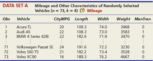
(a). If you did not already do so, rerun the regression requesting variance inflation factors (VIFs) for your predictors.
(b). Do the VIFs suggest that multicollinearity is a problem? Explain.
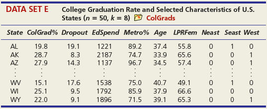
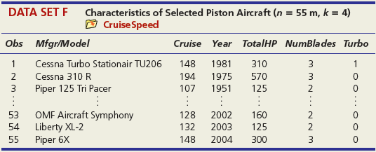


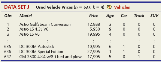
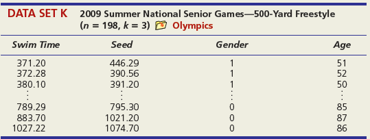
Transcribed Image Text:
DATA SET A Mileage and Other Characteristics of Randomly Selected Vehicles (n = 73, k = 4) O Mileage Obs Vehicle CityMPG Length Width Weight ManTran 3968 3583 1 Acura TL 20 109.3 108.3 74.0 Audi A5 73.0 71.9 2 22 1 BMW 4 Series 428i 22 182.6 3470 Volkswagen Passat SE Volvo S60 T5 71 24 191.6 72.2 3230 72 21 182.2 73.4 3528 73 Volvo XC90 16 189.3 76.2 4667 DATA SET B Noodles & Company Sales, Seating, and Demographic Data (n = 74, k = 5) O Noodles2 Obs Sales/SqFt Seats-Inside Seats-Patio Medincome MedAge Bach Deg% 1 702 66 18 45.2 34.4 31 2 210 69 16 51.9 41.2 20 365 67 10 51.4 40.3 24 72 340 63 28 60.9 43.5 21 73 401 72 15 73.8 41.6 29 74 327 76 24 64.2 31.4 15 DATA SET C = 32, Assessed Value of Small Medical Office Buildings (n = k = 5) O Assessed Obs Assessed Floor Offices Entrances Age Freeway 1 1796 4790 4 2 8 2 1544 4720 3 2 12 3 2094 5940 4 2 2 30 1264 3580 3 2 27 31 1162 3610 2 1 8 1 32 1447 3960 3 2 17 DATA SET D Changes in Consumer Price Index, Capacity Utilization, Changes in Money Supply Components, and Unemployment (n = 41, k = 4) O Money Year ChgCPI СapUtil ChgM1 ChgM2 Unem 1966 2.9 91.1 2.5 4.6 3.8 1967 3.1 87.2 6.6 9.3 3.8 1968 4.2 87.1 7.7 8.0 3.6 2004 2.7 76.6 5.3 5.8 5.5 2005 3.4 78.8 -0.2 4.0 5.1 2006 3.2 80.4 -0.5 5.3 4.6 co co m m m Ln -6 DATA SET E College Graduation Rate and Selected Characteristics of U.S. States (n = 50, k = 8) D ColGrads State ColGrad% Dropout EdSpend Metro% Age LPRFem Neast Seast West AL 19.8 19.1 1221 89.2 37.4 55.8 1 2187 1137 74.7 33.9 34.5 AK 28.7 8.3 65.6 1 AZ 27.9 14.3 96.7 57.4 15.1 17.6 1538 75.0 40.7 49.1 1 WI 25.1 9.5 1792 85.9 37.9 66.6 WY 22.0 9.1 1896 71.5 39.1 65.3 - ... O O- O oo. OOO DATA SET F Characteristics of Selected Piston Aircraft (n = 55 m, k = 4) O CruiseSpeed Obs Mfgr/Model Cruise Year TotalHP NumBlades Turbo 1 Cessna Turbo Stationair TU206 148 1981 310 3 1 2 Cessna 310 R 194 1975 570 3 3 Piper 125 Tri Pacer 107 1951 125 2 OMF Aircraft Symphony Liberty XL-2 Piper 6X 53 128 2002 160 2 54 132 2003 125 2 55 148 2004 300 3. O O... O O o DATA SET G Characteristics of Randomly Chosen Hydrocarbons (n = 35, k = 7) O Retention Obs Name Ret MW ВР RI H1 H2 H3 H4 2,4,4-trimethyl-2-pentene 153.57 1,5-cyclooctadiene methylcyclohexane 1 112.215 105.06 1.4135 1 2 237.56 108.183 150.27 1.4905 1 3 153.57 98.188 101.08 1.4206 ethylbenzene m-ethyl toluene 3-methylhexane 33 209.700 106.170 136.000 1.4950 34 247.800 120.194 161.480 1.4941 35 132.320 100.204 92.000 1.3861 1 O OF... o C O OO... Oo O O O O... O O DATA SET H 2007 Foreclosure' data-toggle="tooltip" data-placement="top" title="Click to view definition...">Foreclosure Rates (n = 50, k = 7) O Foreclosures2 State Foredosure Masslayoff Subprimeshare PricelncomeRatio Ownership 5YrApp UnempChange %HousMoved 28% 18% Alabama 2.70 5.96 4.04 76.6 32.51 0.00% 0.448 Alaska 4.90 2.78 5.54 66.0 53.91 -4.62% 0.426 Arizona 15.20 1.56 26% 6.79 71.1 96.55 -7.32% 0.383 West Virginia 0.50 1.05 21% 4.34 81.3 35.82 -2.13% 0.502 Wisconsin 4.90 12.50 21% 4.83 71.1 36.37 4.26% 0.428 Wyoming 1.50 0.96 23% 5.06 72.8 62.56 -9.09% 0.498 DATA SET I Body Fat and Personal Measurements for Males (n = 50, k = 8) O BodyFat2 Obs Fat% Age Weight Height Neck Chest Abdomen Hip Thigh 1 12.6 23 154.25 67.75 36.2 93.1 85.2 94.5 59.0 6.9 22 173.25 72.25 38.5 93.6 83.0 98.7 58.7 3 24.6 22 154.00 66.25 34.0 95.8 87.9 99.2 59.6 48 6.4 39 148.50 71.25 34.6 89.8 79.5 92.7 52.7 49 13.4 45 135.75 68.50 32.8 92.3 83.4 90.4 87.2 52.0 50 5.0 47 127.50 66.75 34.0 83.4 70.4 50.6 DATA SET J Used Vehicle Prices (n = 637, k = 4) O Vehicles Obs Model Price Age Car Truck SUV Astro GulfStream Conversion 12,988 5,950 19,995 1 3 Astro LS 4.3L V6 9. Astro LS V6 4. DC 300M Autostick DC 300M Special Edition GM 3500 4x4 w/8ft bed and plow 17,995 635 10,995 22,995 6. 636 1 1 637 5 1 OO O. .. O O O DATA SET K 2009 Summer National Senior Games-500-Yard Freestyle (n = 198, k = 3) D olympics Swim Time Seed Gender Age 371.20 446.29 390.56 391.20 1 51 52 372.28 380.10 50 789.29 795.30 85 883.70 1027.22 1021.20 1074.70 87 86 - -.. 000
> Using the “Metals” data, construct a correlation matrix of the six independent variables. The response variable is Priceylb. (a). Identify any pairs of independent variables that have a significant pairwise correlation. (b). Using MegaStat or MINITAB,
> (a) Use Excel to make a scatter plot of the data. (b) Select the data points, right-click, select Add Trendline, select the Options tab, and choose Display equation on chart and Display R-squared value on chart. (c) Interpret the fitted slope. (d) Is the
> (a) Use Excel to make a scatter plot of the data. (b) Select the data points, right-click, select Add Trendline, select the Options tab, and choose Display equation on chart and Display R-squared value on chart. (c) Interpret the fitted slope. (d) Is the
> (a) Make an Excel worksheet to calculate SSxx, SSyy, and SSxy (the same worksheet you used in exercises 12.2 and 12.3). (b) Use the formulas to calculate the slope and intercept. (c) Use your estimated slope and intercept to make a worksheet to calculate
> (a) Make an Excel worksheet to calculate SSxx, SSyy, and SSxy (the same worksheet you used in exercises 12.2 and 12.3). (b) Use the formulas to calculate the slope and intercept. (c) Use your estimated slope and intercept to make a worksheet to calculate
> Refrigerator prices are affected by characteristics such as whether or not the refrigerator is on sale, whether or not it is listed as a Sub-Zero brand, the number of doors (one door or two doors), and the placement of the freezer compartment (top, side,
> A regression model to predict the price of diamonds included the following predictor variables: the weight of the stone (in carats where 1 carat = 0.2 gram), the color rating (D, E, F, G, H, or I), and the clarity rating (IF, VVS1, VVS2, VS1, or VS2). (
> Which statement is false? Explain. a. If μ = 52 and σ = 15, then X = 81 would be an outlier. b. If the data are from a normal population, about 68 percent of the values will be within μ ± σ. c. If μ = 640 and σ = 128 then the coefficient of variation is
> (a) Does the 95 percent confidence interval for the slope include zero? If so, what does this tell you? If not, what does it mean? (b) Do a two-tailed t test for zero slope at α = .05. State the hypotheses, degrees of freedom, and critical
> Below are fitted regressions for Y = asking price of a used vehicle and X = the age of the vehicle. The observed range of X was 1 to 8 years. The sample consisted of all vehicles listed for sale in a particular week. (a) Interpret the slope of each fitte
> The regression equation Credits = 15.4 -.07 Work was estimated from a sample of 21 statistics students. Credits is the number of college credits taken and Work is the number of hours worked per week at an outside job. (a). Interpret the slope. (b). Is
> The regression equation HomePrice = 51.3 + 2.61 Income was estimated from a sample of 34 cities in the eastern United States. Both variables are in thousands of dollars. HomePrice is the median selling price of homes in the city, and Income is median fam
> The regression equation NetIncome = 2,277 + .0307 Revenue was estimated from a sample of 100 leading world companies (variables are in millions of dollars). (a). Interpret the slope. (b). Is the intercept meaningful? Explain. (c). Make a prediction o
> (a) Interpret the slope of the fitted regression Number of International Franchises = -47.5 + 1.75 Power Distance Index. The Power Distance Index is a measure on a scale of 0–100 of the wealth gap between the richest and poorest in a country. (b) What is
> Observations are taken on sales of a certain mountain bike in 30 sporting goods stores. The regression model was Y = total sales (thousands of dollars), X1 = display floor space (square meters), X2 = competitors’ advertising expenditure
> Observations are taken on net revenue from sales of a certain LCD TV at 50 retail outlets. The regression model was Y = net revenue (thousands of dollars), X1 = shipping cost (dollars per unit), X2 = expenditures on print advertising (thousands of dollar
> Refer to the ANOVA table below. (a) State the degrees of freedom for the F test for overall significance. (b) Use Appendix F to look up the critical value of F for α = .05. (c) Calculate the F statistic. Is the regression significant overal
> (a) Make a scatter plot of the data. What does it suggest about the correlation between X and Y? (b) Use Excel, MegaStat, or MINITAB to calculate the correlation coefficient. (c) Use Excel or Appendix D to find t.025 for a two-tailed test at Î&plu
> (a) Make an Excel scatter plot. What does it suggest about the population correlation between X and Y? (b) Make an Excel worksheet to calculate SSxx, SSyy, and SSxy. Use these sums to calculate the sample correlation coefficient. Check your work by using
> Use Excel, MegaStat, or MINITAB to fit the regression model, including residuals and standardized residuals. Midterm and Final Exam Scores for Business Statistics Students Fall Semester 2011 (n = 58 students) Midterm Exam Score …&ac
> Which statement is true? Why not the others? a. We expect the median to exceed the mean in positively skewed data. b. The geometric mean is not possible when there are negative data values. c. The midrange is resistant to outliers.
> For each sample, do a test for zero correlation. (a) Use Appendix D to find the critical value of tα. (b) State the hypotheses about ρ. (c) Perform the t test and report your decision. Appendix D: a. r = +.45, n = 20, Î&
> A box of Wheat Chex cereal is to be filled to a mean weight of 466 grams. The lower specification limit is 453 grams (the labeled weight is 453 grams) and the upper specification limit is 477 grams (so as not to overfill the box). The process standard de
> A new type of smoke detector battery is developed. From laboratory tests under standard conditions, the half-life (defined as less than 50 percent of full charge) of 20 batteries are shown below. (a). Make a histogram of the data and/or a probability p
> A Nabisco Fig Newton has a process mean weight of 14.00 g with a standard deviation of 0.10 g. The lower specification limit is 13.40 g and the upper specification limit is 14.60 g. (a). Describe the capability of this process, using the techniques you
> Refer to the freezer data’s 80 individual temperature observations in problem 17.52. Problem 17.52: Refer to the freezer problem 17.51 with μ = 23 and σ = 2. Temperature measurements are recorded four times a
> The temperature control unit on a commercial freezer in a 24-hour grocery store is set to maintain a mean temperature of 23 degrees Fahrenheit. The temperature varies because people are constantly opening the freezer door to remove items, but the thermos
> Refer back to Table 15.11, which shows the distribution of the number of U.S. Supreme Court appointments per year from 1900–1999. Since 1999 there have been four Supreme Court appointments with one each in the years 2005, 2006, 2009, an
> (a) Use Excel’s Data Analysis > Random Numbers to generate 100 Poisson-distributed random numbers with a mean of λ = 4. (b) Make a histogram of your sample and assess its shape. (c) Calculate descriptive statistics. Are
> (a) Use Excel’s function =RAND() or Excel’s Data Analysis > Random Numbers to generate 100 uniformly distributed random numbers between 0 and 1. (b) Make a histogram of your sample and assess its shape. (c) Calculat
> Interpret the slope. Does the intercept have meaning, given the range of the data? Midterm and Final Exam Scores for Business Statistics Students Fall Semester 2011 (n = 58 students) Midterm Exam Score ……â&
> (a) Use Excel’s function =NORM.INV(RAND(),0,1) or Excel’s Data Analysis > Random Numbers to generate 100 normally distributed random numbers with a mean of 0 and a standard deviation of 1. (b) Make a histogram of yo
> If a random experiment whose success probability is .20 is repeated 8 times, find the probability of (a) exactly 3 successes; (b) more than 3 successes; (c) at most 2 successes. (d) Which probability distribution did you use and why?
> Using test data on 43 vehicles, an analyst fitted a regression to predict CityMPG (miles per gallon in city driving) using as predictors Length (length of car in inches), Width (width of car in inches), and Weight (weight of car in pounds). Interpret the
> Analysis of a Detroit Marathon (n = 1,015 men, n = 150 women) produced the regression results shown below, with dependent variable Time (the marathon time in minutes) and predictors Age (runner’s age), Weight (runner’s
> An expert witness in a case of alleged racial discrimination in a state university school of nursing introduced a regression of the determinants of Salary of each professor for each year during an 8-year period (n = 423) with the following results, with
> A sports enthusiast created an equation to predict Victories (the team’s number of victories in the National Basketball Association regular season play) using predictors FGP (team field goal percentage), FTP (team free throw percentage)
> A researcher used stepwise regression to create regression models to predict Birth Rate (births per 1,000) using five predictors: LifeExp (life expectancy in years), InfMort (infant mortality rate), Density (population density per square kilometer), GDPC
> Using test data on 20 types of laundry detergent, an analyst fitted a regression to predict Cost Per Load (average cost per load in cents per load) using binary predictors Top Load (1 if washer is a top loading model, 0 otherwise) and Powder (if detergen
> A hospital emergency room analyzed n = 17,664 hourly observations on its average occupancy rates using six binary predictors representing days of the week and two binary predictors representing the 8-hour work shift (12 a.m.–8 a.m., 8 a.m.–4 p.m., 4 p.m.
> In a study of paint peel problems, a regression was suggested to predict defects per million (the response variable). The intended predictors were supplier (four suppliers, coded as binaries) and substrate (four materials, coded as binaries). There were
> Which one of the following is true? Why not the others? a. Histograms are useful for visualizing correlations. b. Pyramid charts are generally preferred to bar charts. c. A correlation coefficient can be negative.
> In a model of Ford’s quarterly revenue Total Revenue = β0 + β1 Car Sales + β2 Truck Sales + β3 SUVSales + ε, the three predictors are measured in number of units sold (not dollars). (a). Interpret each slope. (b). Would the intercept be meaningful? (c)
> If you are using time-series data, perform one or more tests for autocorrelation (visual inspection of residuals plotted against observation order, runs test, Durbin-Watson test). Is autocorrelation a concern? DATA SET A Mileage and Other
> Here are the ages of a random sample of 20 CEOs (chief executive officers) of Fortune 500 U.S. corporations. (a). Find the mean, median, and mode. (b). Discuss advantages and disadvantages of each of these measures of center for this data set. (c). F
> If you did not already do so, request a plot of residuals versus the fitted Y. Is heteroscedasticity a concern? DATA SET A Mileage and Other Characteristics of Randomly Selected Vehicles (n = 73, k = 4) O Mileage Obs Vehicle CityMPG Length
> If you did not already do so, request a histogram of standardized residuals and/or a normal probability plot. Do the residuals suggest non-normal errors? Explain. DATA SET A Mileage and Other Characteristics of Randomly Selected Vehicles (
> If you did not already do so, request leverage statistics. Are any observations influential? Explain. DATA SET A Mileage and Other Characteristics of Randomly Selected Vehicles (n = 73, k = 4) O Mileage Obs Vehicle CityMPG Length Width Wei
> (a). If you did not already do so, request a table of standardized residuals. (b). Are any residuals outliers (three standard errors) or unusual (two standard errors)? DATA SET A Mileage and Other Characteristics of Randomly Selected Vehi
> (a). Generate a correlation matrix for your predictors. Round the results to three decimal places. (b). Based on the correlation matrix, is collinearity a problem? DATA SET A Mileage and Other Characteristics of Randomly Selected Vehicles
> Use the standard error to construct an approximate prediction interval for Y. Based on the width of this prediction interval, would you say the predictions are good enough to have practical value? DATA SET A Mileage and Other Characteristi
> Use Excel’s Add Trendline feature to fit a linear regression to the scatter plot. Is a linear model credible? Midterm and Final Exam Scores for Business Statistics Students Fall Semester 2011 (n = 58 students) Midterm Exam Score &acir
> Based on the R2 and ANOVA table for your model, how would you describe the fit? DATA SET A Mileage and Other Characteristics of Randomly Selected Vehicles (n = 73, k = 4) O Mileage Obs Vehicle CityMPG Length Width Weight ManTran 3968 3583
> (a) Which p-values indicate predictor significance at α = .05? (b) Do the p-values support the conclusions you reached from the t tests? (c) Do you prefer the t test or the p-value approach? Why? DATA SET A Mileage and Other
> (a) Plot U.S. petroleum imports on a graph. (b) Describe the trend (if any) and discuss possible causes. (c) Fit both a linear and an exponential trend. (c) Interpret each fitted trend equation, explaining the implications. (d) Make a projection for 2010
> (a) Plot both men’s and women’s winning times on the same graph. (b) Fit a linear trend model to each series (men, women). (c) Use Excel’s option to forecast each trend graphically to 2040 (i.e., to p
> Do a two-tailed t test for zero slope for each predictor coefficient at α = .05. State the degrees of freedom and look up the critical value in Appendix D (or from Excel). Appendix D: Confidence Level Confidence Level 80 90
> Does a class break stimulate the pulse? Here are heart rates for a sample of 30 students before and after a class break. Research question: At α = .05, do the medians differ? Heart Rate before and after Class Break Student Before After
> Salaries of 30 randomly chosen individuals in the same occupation (only the first 3 and last 3 observations are shown). The data are from a salary equity study comparing two industries. Research question: Without assuming normality of the populations, is
> (a) Plot the data on law enforcement officers killed. (b) Describe the trend (if any) and discuss possible causes or anomalies in the data. (c) Would a fitted trend be helpful? Explain. (c) Make a forecast for 2009 using any method you like (including ju
> A cognitive retraining clinic assists outpatient victims of head injury, anoxia, or other conditions that result in cognitive impairment. Each incoming patient is evaluated to establish an appropriate treatment program and estimated length of stay (ELOS
> (a) Plot both men’s and women’s winning times on the same graph. (b) Fit a linear trend model to each series. From the fitted trends, will the times eventually converge? Hint: Ask Excel for forecasts (e.g., 20 years ah
> (a) Plot either receipts and outlays or federal debt and GDP (plot both time series on the same graph). (b) Describe the trend (if any) and discuss possible causes. (c) Fit a trend of your choice to each. (d) Interpret each fitted trend equation, explain
> (a) Choose one beverage category and plot the data. (b) Describe the trend (if any) and discuss possible causes. (c) Would a fitted trend be helpful? Explain. (d) Fit several trend models. Which is best, and why? If none is satisfactory, explain. (e) Mak
> (a) Plot the data on U.S. general aviation shipments. (b) Describe the pattern and discuss possible causes. (c) Would a fitted trend be helpful? Explain. (d) Make a similar graph for 1993–2008 only. Would a fitted trend be helpful in ma
> Which statement is correct? Why not the others? a. Likert scales are interval if scale distances are meaningful. b. Cross-sectional data are measured over time. c. A census is always preferable to a sample.
> (a) Choose one category of consumer credit and plot it. (b) Describe the trend (if any) and discuss possible causes. (c) Fit a trend model of your choice. (d) Make forecasts for 3 years (2011–2013), using a trend model of your choice.
> If freeway speeds are normally distributed with a mean of μ = 70 mph and σ = 7 mph, find the probability that the speed of a randomly chosen vehicle (a) exceeds 78 mph; (b) is between 65 and 75 mph; (c) is less than 70 mph.
> (a) Plot the voter participation rate. (b) Describe the trend (if any) and discuss possible causes. (c) Fit both a linear and a quadratic trend to the data. (d) Which model is preferred? Why? (e) Make a forecast for 2012, using a trend model of your choi
> (a) Plot the total minutes of TV viewing time per household. (b) Describe the trend (if any) and discuss possible causes. (c) Fit a linear trend to the data. (d) Would this model give reasonable forecasts? Would another trend model be better? Explain. (e
> (a) Plot both Swiss watch time series on the same graph. (b) Describe the trend (if any) and discuss possible causes. (c) Fit an exponential trend to each time series. (d) Interpret each fitted trend carefully. What conclusion do you draw? (e) Make forec
> (a) Make a line chart for JetBlue’s revenue. (b) Describe the trend (if any) and discuss possible causes. (c) Fit both a linear and an exponential trend to the data. (d) Which model is preferred? Why? (e) Make annual forecasts for 2011&
> Fertility rates (children born per woman) are shown for 27 EU member nations in 2 years. Research question: At α = .05, is there a significant rank correlation? Only the first 3 and last 3 nations are shown. Fertility Rates in EU Membe
> The table below shows annual financial data for a sample of 20 companies in the food consumer products sector. Research question: At α = .01, is there a significant correlation between revenue and profit? Why is a rank correlation preferred
> In a call center, the average waiting time for an answer (in seconds) is shown below by time of day. Research question: At α = .01, does the waiting time differ by day of the week? Only the first 3 and last 3 observations are shown. Av
> Below are results of braking tests of a certain SUV on glare ice, packed snow, and split traction (one set of wheels on ice, the other on dry pavement), using three braking methods. Research question: At α = .01, is braking method related t
> Mean output of arrays of solar cells of three types are measured four times under random light intensity over a period of 5 minutes, yielding the results shown below. Research question: At α = .05, is the median solar cell output the same f
> Which of the following is not a reason for sampling? Explain. a. The destructive nature of some tests. b. High cost of studying the entire population. c. The expense of obtaining random numbers.
> Does the 95 percent confidence interval for each predictor coefficient include zero? What conclusion can you draw? DATA SET A Mileage and Other Characteristics of Randomly Selected Vehicles (n = 73, k = 4) O Mileage Obs Vehicle CityMPG Len
> The waiting time (in minutes) for emergency room patients with non-life-threatening injuries was measured at four hospitals for all patients who arrived between 6:00 and 6:30 p.m. on a certain Wednesday. The results are shown below. Research question: At
> In a bumper test, three types of autos were deliberately crashed into a barrier at 5 mph, and the resulting damage (in dollars) was estimated. Five test vehicles of each type were crashed, with the results shown below. Research question: At Î&plusm
> Below are grade point averages for 25 randomly chosen university business students during a recent semester. Research question: At α = .01, are the median grade point averages the same for students in these four class levels? Grade Poi
> The square footage of each of the last 11 homes sold in each of two suburban neighborhoods is noted. Research question: At α = .01, do the medians differ? Square Footage of Homes Sold Grosse Hills (Built in 1985) Grosse Hills Haut Nez
> Adult height is somewhat predictable from average height of both parents. For females, a commonly used equation is YourHeight = ParentHeight - 2.5 while for males the equation is YourHeight = ParentHeight + 2.5. (a). Test these equations on yourself an
> Below are results of a regression of Y = average stock returns (in percent) as a function of X = average price/earnings ratios for the period 1949–1997 (49 years). Separate regressions were done for various holding periods (sample sizes
> Below are fitted regressions based on used vehicle ads. Observed ranges of X are shown. The assumed regression model is AskingPrice = f (VehicleAge). (a). Interpret the slopes. (b). Are the intercepts meaningful? Explain. (c). Assess the fit of each
> Below are revenue and profit (both in $ billions) for nine large entertainment companies. (a). Make a scatter plot of profit as a function of revenue. (b). Use Excel to fit the regression, with fitted equation and R2. (c). In your own words, describ
> A common belief among faculty is that teaching ratings are lower in large classes. Below are MINITAB results from a regression using Y = mean student evaluation of the professor and X = class size for 364 business school classes taught during the 2002&ac
> An experimental bumper was designed to reduce damage in low-speed collisions. This bumper was installed on an experimental group of vans in a large fleet, but not on a control group. At the end of a trial period, accident data showed 12 repair incidents
> Perform the regression and write the estimated regression equation (round off to 3 or 4 significant digits for clarity). Do the coefficient signs agree with your a priori expectations? DATA SET A Mileage and Other Characteristics of Random
> (a) Interpret the slope of the fitted regression HomePrice = 125,000 + 150 SquareFeet. (b) What is the prediction for HomePrice if SquareFeet = 2,000? (c) Would the intercept be meaningful if this regression applies to home sales in a certain subdivision
> Two manufacturing facilities produce 1280 × 1024 LED (light-emitting diode) displays. Twelve shipments are tested at random from each lab, and the number of bad pixels per billion is noted for each shipment. Research question: At Î&plu
> Simple regression was employed to establish the effects of childhood exposure to lead. The effective sample size was about 122 subjects. The independent variable was the level of dentin lead (parts per million). Below are regressions using various depend
> Choose one of these three data sets. (a) Make a scatter plot. (b) Let Excel estimate the regression line, with fitted equation and R2. (c) Describe the fit of the regression. (d) Write the fitted regression equation and interpret the slope. (e) Do you th
> Consider the following Excel regression of perceived sound quality as a function of price for 27 stereo speakers. (a) Is the coefficient of Price significantly different from zero at α = .05? (b) What does the R2 tell you? (c) Given these r
> Below are fertility rates (average children born per woman) in 15 EU nations for 2 years. (a) Make a scatter plot. (b) Find the correlation coefficient and interpret it. (c) Test the correlation coefficient for significance, clearly stating the degrees o
> Below are percentages for annual sales growth and net sales attributed to loyalty card usage at 74 Noodles & Company restaurants. (a) Make a scatter plot. (b) Find the correlation coefficient and interpret it. (c) Test the correlation coefficient for
> Do stock prices of competing companies move together? Below are daily closing prices of two computer services firms (IBM = International Business Machines Corporation, HPQ = Hewlett- Packard Company. (a) Calculate the sample correlation coefficient (e.g.
> In the following regression, X = total assets ($ billions), Y = total revenue ($ billions), and n = 64 large banks. (a) Write the fitted regression equation. (b) State the degrees of freedom for a two tailed test for zero slope, and use Appendix D to fin
> In the following regression, X = monthly maintenance spending (dollars), Y = monthly machine downtime (hours), and n = 15 copy machines. (a) Write the fitted regression equation. (b) State the degrees of freedom for a two-tailed test for zero slope, and

