Question: Background Information: Restaurants have
Background Information: Restaurants have traditionally used bottom-end wines to sell by the glass (BTG) at reasonably low prices per glass. In recent years, there has been a growing trend within the restaurant industry to extend BTG programs to higher-end wines. In doing so, they have greatly expanded the sales of higher-end wines. The typical markup on a bottle of wine is 100 percent or more, meaning that a bottle of wine that sells at retail for $25 in a wine shop can be priced at $100 in a restaurant. To simplify this discussion, suppose that wine is offered at $10 per glass. The size of the serving can be adjusted depending on the price per bottle of the wine being poured. For example, a 4-ounce pour can be offered for wines in the $40 to $50 range and a 2-ounce pour can be offered for wines in the $80 to $100 range. Because a bottle has 25.4 ounces, both examples provide more revenue from BTG sales than from full-bottle sales! Such programs have been quite successful and produce little loss due to unsold wine in the bottle because, with proper storage, a partial bottle can be poured the next evening with no notable change in taste.
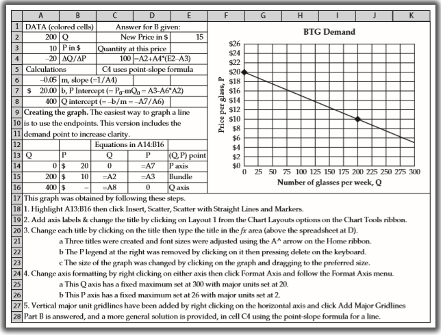
The Problem: Suppose you manage a restaurant with a BTG program. You sell 200 glasses per week at $10 per glass. As an experiment, you once raised the price during the week to $11 a glass and found that you sold 20 glasses less than before the price change. Suppose you assume this information as the basis for a full demand curve for wine BTG at your restaurant.
a. Obtain an algebraic and graphical depiction of your restaurant’s BTG demand.
b. How many glasses do you expect to sell at $15 per glass?
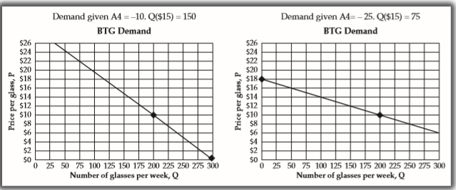
c. How would your answers change if the response to a $1 price change is 10 glasses per week or 25 glasses per week?
We now demonstrate how Excel can be used to answer this problem. This allows you to easily conduct a what-if or sensitivity analysis. It also prepares you to use Excel to analyze and estimate more complex demand relationships such as those presented in Chapters 4 and 5. Note: This problem requires three important assumptions.
1. You know a point on the BTG demand curve (e.g., P = $10 and Q = 200).
2. You know the slope of the BTG demand curve at this point is ∆P/∆Q = .05.
3. You know that the slope does not change (i.e., demand for wine BTG is linear). For a review of slopes and equations, go to the Mathematical Appendix on the Companion Website or see Appendix 3A.
Excel Sheet 3.1 shows a screenshot of cells A1:K28 from the Single Demand worksheet of the Demand Excel App. It shows one way to analyze this problem in Excel. The graph is shown next to calculations, and equations are shown next to critical cells, in the worksheet. This is simply done to clarify how each number was obtained: By clicking on a cell, you can check the equations for yourself. This example provides a detailed roadmap for creating a graph in Excel. You are encouraged to open Excel and do this problem yourself.
Notice that the negative slope of the demand curve is represented by the negative sign in cell A4 rather than by writing the equation as P = b - mQ. Both practices work as long as
Excel Sheet 3.1
Source: Demand Excel App, Single Demand worksheet.
Alternate Figures from Excel Sheet 3.1 based on Changing Demand Responsiveness in Cell A4 you follow through with the mathematics consistently. The benefit of not forcing the minus sign into the equation is that a supply curve can readily be modeled with this graph by entering a positive slope in cell A4. Of course, you also want to adjust the labels appropriately.
One quick benefit of doing the problem in Excel is that the new scenarios in part c are analyzed by changing a single cell, A4, on Excel Sheet 3.1(the figures below are from Excel Sheet 3.1 based on new values for A4). Additional scenarios can be examined by varying any of the four pieces of data on which the problem is based (in cells A2:A4 and E2 on Excel Sheet 1).
Transferring Your Excel Work to Other Programs: Once you have a graph you want to use, you can easily insert it into another program by highlighting the graph in Excel and then using the Copy command on Excel’s Home ribbon. To paste in a Word or PowerPoint document, open that software and use Paste Special, Enhanced Metafile, rather than Paste. From this point, the graph can be resized or positioned as needed by right-clicking on the image; it can be adjusted as needed using the Size and Format Picture menus.
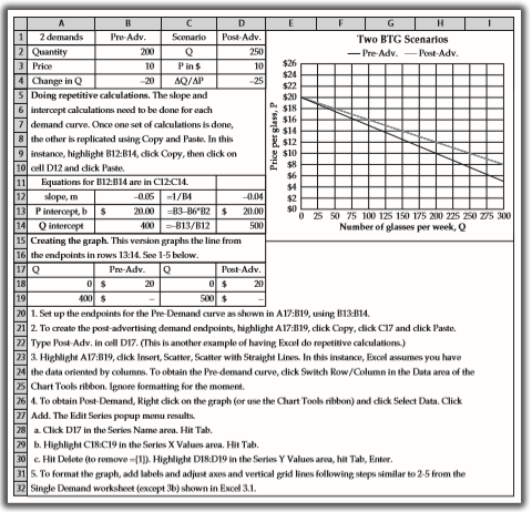
Here is a second, related problem: A successful advertising campaign has increased BTG demand by 25 percent at any price relative to pre-advertising levels. Pre-advertising demand is assumed to be the same as was given in the initial 1Demand scenario (200 glasses are sold at a price of $10 per glass, and each dollar price change is associated with a twenty glass-per-week change in sales).
The post advertising demand implies that 250 glasses are sold at a price of $10 per glass, and each dollar price change is associated with a twenty-five-glass-per-week change in sales. This is confirmed by having the P intercept the same for both demand curves. Excel Sheet 3.2 shows how this is analyzed in Excel.
One final scenario: Try doing this problem yourself using the worksheet you created or the 2Demands worksheet. Consider an alternative post advertising scenario. Rather than selling 25 percent more glasses at any price, you find that if you charge 25 percent more per glass, then you are able to maintain the same number of BTG glasses sold. Adjust D2:D4 to model this new scenario and Copy and Paste (using Paste-Special as described above) your answer graph to a fresh sheet of paper; include answers to a and b:
a. Provide a verbal description of demand in this instance by filling in the values of C and D in the following sentence: Post advertising demand shows that 200 glasses are sold at a price of C per glass, and each dollar price change is associated with a D-glass-per-week change in sales.
b. What is the equation for the post advertising demand curve in slope-intercept form?
Excel Sheet 3.2
Source: Demand Excel App, Multiple Demands worksheet
Transcribed Image Text:
A 1 DATA (colored cells) 200 Q Answer for B given: BTG Demand 2 New Price in $ 15 $26 $24 Quantity at this price 100 -A2+A4'(E2-A3) C4 uses point-slope formula 10 Pin $ -20 AQ/AP $22 5 Calculations -0.05 m, slope (-1/A4) $ 20.00 b, P Intercept (= Pg-mQg = A3-A6°A2) 400 Qintercept (=-b/m =-A7/A6) 9 Creating the graph. The easiest way to graph a line 10 is to use the endpoints. This version includes the 11 demand point to increase clarity. $20 A $18 I $16 $14 7 8 $12 * $10 $8 Equations in A14:B16 P. $6 $4 12 (QP) point Paxis Bundle Qaxis 13 Q $2 $0 O 25 50 75 100 125 150 175 200 225 250 275 300 14 20 =A7 15 200 $ 10 =A2 =A3 Number of glasses per week, Q 16 400 $ A8 17 This graph was obtained by following these steps. 18 1. Highlight A13:B16 then click Insert, Scatter, Scatter with Straight Lines and Markers. 19 2. Add axis labels & change the title by clicking on Layout 1 from the Chart Layouts options on the Chart Tools ribbon. 20 3. Change each title by clicking on the title then type the title in the fx area (above the spreadsheet at D). 21 a Three titles were created and font sizes were adjusted using the A^ arrow on the Home ribbon. b The Plegend at the right was removed by clicking on it then pressing delete on the keyboard. c The size of the graph was changed by clicking on the graph and dragging to the preferred size. 22 23 24 4. Change axis formatting by right clicking on either axis then click Format Axis and follow the Format Axis menu. 25 a This Qaxis has a fixed maximum set at 300 with major units set at 20. b This P axis has a fixed maximum set at 26 with major units set at 2. 26 27 5. Vertical major unit gridlines have been added by right clicking on the horizontal axis and click Add Major Gridlines 28 Part B is answered, and a more general solution is provided, in cell CA using the point-slope formula for a line. Price per glass, P Demand given A4 =-10. Q($15) = 150 Demand given A4=- 25. Q($15) = 75 BTG Demand BTG Demand $26 $24 $22 $20 $18 $16 $14 $26 $24 $22 $20 $18 $16 $14 $12 $10 $8 $6 $4 $2 $0 $12 $10 $8 $6 $4 $2 $0 O 25 50 75 100 125 150 175 200 225 250 275 300 O 25 50 75 100 125 150 175 200 225 250 275 300 Number of glasses per week, Q Number of glasses per week, Q Price per glass, P Price per glass, P B D 1 2 demands Pre Adv. Scenario Past-Adv. Two BTG Scenarios 2 Quantity 3 Price 200 250 - Pre-Adv. -Post-Adv. $26 $24 $22 $20 $18 $16 10 Pin$ 10 4 Change in Q 5 Doing repetitive calculations. The slope and 6 intercept caleulations need to be done for each 7 demand curve. Once one set of calculations is done, 8 the other is replicated using Copy and Paste. In this 9 instance, highlight B12:B14, dick Copy, then dick on 10 cell D12 and dick Paste. 11 20 AQ/AP -25 $14 $12 $10 $6 Equations for Bl2:B14 are in C12C14. -0.05 -1/B4 $4 12 13 Pintercept, b s Q intercept slope, m -0.04 $2 $0 O 25 50 75 100 125 150 175 200 225 250 275 300 Number of glasses per week, Q 20.00 =83-B6"B2 $ 20.00 14 400 -B13/B12 500 15 Creating the graph. This version graphs the line from 16 the endpoints in rows 13:14. See 1-5 bekow. 17 Q Pre-Adv. Post-Adv. 18 20 20 19 400 S 500 $ 20 1. Set up the endpoints for the Pre-Demand curve as shown in A17:B19, using B13-B14. 21 2 To create the post-advertising demand endpoints, highlight A17:B19, dick Copy, dick C17 and click Paste. 22 Type Post-Adv. in cell DI7. (This is another example of having Excol do repetitive calculations.) 23 3. Highlight A17:B19, dick Insort, Scatter, Scatter with Straight Lines. In this instance, Excel assumes you have 24 the data oriented by columns. To obtain the Pre-demand curve, dick Switch Row/Column in the Data area of the 25 Chart Tools ribbon. Ignore formating for the moment. 26 4. To obtain Post-Demand, Right dick on the graph (or use the Chart Tools ribbon) and dick Select Data. Click 27 Add. The Edit Series popup menu results. 78 a. Click D17 in the Series Name area. Hit Tab. 29 b. Highlight Cl18:C19 in the Sories X Values area. Hit Tab. 30 c. Hit Delote (to romove -(1). Highlight D18:D19 in the Series Y Values area, hit Tab, Enter. 31 5. To format the graph, add labels and adjust axes and vertical grid lines following steps similar to 2-5 from the 32 Single Demand worksheet (except 3b) shown in Excel 3.1. d'ss8 sad aopa
> The compound growth rate is frequently used to forecast various quantities (sales, profits, and so on). Do you believe this is a good method? Should any cautions be exercised in making such projections?
> Discuss some of the important criticisms of the forecasting ability of the leading economic indicators.
> a. Why are manufacturers’ new orders, nondefense capital goods, an appropriate leading indicator? b. Why is the index of industrial production an appropriate coincident indicator? c. Why is the average prime rate charged by banks an appropriate lagging i
> Discuss the benefits and drawbacks of the following methods of forecasting: a. Jury of executive opinion b. The Delphi method c. Opinion polls Each method has its uses. What are they?
> Enumerate methods of qualitative and quantitative forecasting. What are the major differences between the two?
> “The best forecasting method is the one that gives the highest proportion of correct predictions.” Comment.
> What is the identification problem? What effect will this problem have on the regression estimates of a demand function? Explain.
> What is multicollinearity? How can researchers detect this problem? What is the impact of this problem on the regression estimates? What steps can be taken to deal with this problem?
> A book store opens across the street from the University Book Store (UBS). The new store carries the same textbooks but offers a price 20 percent lower than UBS. If the cross- price elasticity is estimated to be 1.5, and UBS does not respond to its compe
> The ABC marketing consulting firm found that a particular brand of tablet PCs has the following demand curve for a certain region: Q = 10,000 - 200P + 0.03Pop + 0.6I + 0.2A where Q is the quantity per month, P is price ($), Pop is population, I is dispos
> In the Columbia Gas of Ohio study that forecasted the demand for gas (see p. 155), the company developed the following coefficients for their equation: Growth rate ………………………………………………………….015 Intercept…………………………………………………………...1376.0 Forecasted temperatur
> Based on past data, Mack’s Pool Supply has constructed the following equation for the sales of its house brand of chlorine tablets: Q = 1,000 + 100t where Q is quantity and t is time (in years), with 2007 = 0. a. What is the sales projection for 2013? b.
> If the sales of your company have grown from $500,000 five years ago to $1,050,150 this year, what is the compound growth rate? If you expect your sales to grow at a rate of 10 percent for the next five years, what should they be five years from now?
> The MNO Corporation is preparing for its stockholder meeting on May 15, 2013. It sent out proxies to its stockholders on March 15 and asked stockholders who plan to attend the meeting to respond. To plan for a sufficient number of information packages to
> An economist has estimated the sales trend line for the Sun Belt Toy Company as follows: St = 43.6 + 0.8t St represents Sun Belt’s monthly sales (in millions of dollars), and t = 1 in January 2008. The monthly seasonal indexes are as fo
> Office Enterprises (OE) produces a line of metal office file cabinets. The company’s economist, having investigated a large number of past data, has established the following equation of demand for these cabinets: Q = 10,000 + 60B - 100P + 50C where Q 5
> You have the following data for the last 12 months’ sales for the PRQ Corporation (in thousands of dollars): a. Calculate a 3-month centered moving average. b. Use this moving average to forecast sales for January of next year. c. If
> The Miracle Corporation had the following sales during the past 10 years (in thousands of dollars): a. Calculate a trend line, and forecast sales for 2013. How confident are you of this forecast? b. Use exponential smoothing with a smoothing factor w =
> The sales data over the last 10 years for the Acme Hardware Store are as follows: a. Calculate the compound growth rate for the period of 2003 to 2012. b. Based on your answer to part a, forecast sales for both 2013 and 2014. c. Now calculate the compo
> The sales data for the Lone star Sports Apparel Company for the last 12 years are as follows: a. What is the 2001–2012 compound growth rate? b. Using the result obtained in part a, what is your 2013 projection? c. If you were to make
> The following relations describe monthly demand and supply for a computer support service catering to small businesses. QD = 3,000 - 10P QS = -1,000 + 10P where Q is the number of businesses that need services and P is the monthly fee, in dollars. a. At
> You are given the following demand for European luxury automobiles: Q 5 1,000P 20.93PA0.75PJ1.2I 1.6 where P 5 Price of European luxury cars PA 5 Price of American luxury cars PJ 5 Price of Japanese luxury cars I 5 Annual income of car buyers Assume that
> A manufacturer of computer workstations gathered average monthly sales figures from its 56 branch offices and dealerships across the country and estimated the following demand for its product: Q = +15,000 - 2.80P + 150A + 0.3Ppc + 0.35Pm + 0.2Pc (5,234)
> The maker of a leading brand of low-calorie microwavable food estimated the following demand equation for its product using data from 26 supermarkets around the country for the month of April: Q = -5,200 - 42P + 20PX + 5.2l + 0.20A + 0.25M (2.002) (17.5)
> You are the manager of a large automobile dealership who wants to learn more about the effectiveness of various discounts offered to customers over the past 14 months. Following are the average negotiated prices for each month and the quantities sold of
> One of the most difficult tasks in regression analysis is to obtain the data suitable for quantitative studies of this kind. Suppose you are trying to estimate the demand for home furniture. Suggest the kinds of variables that could be used to represent
> The Efficient Software Store had been selling a spreadsheet program at a rate of 100 per month and a graphics program at the rate of 50 per month. In September 2012, Efficient’s supplier lowered the price for the spreadsheet program, and Efficient passed
> The Mesa Redbirds football team plays in a stadium with a seating capacity of 80,000. However, during the past season, attendance averaged only 50,000. The average ticket price was $30. If price elasticity is −4, what price would the team have to charge
> The ABC Company manufactures digital clock radios and sells on average 3,000 units monthly at $25 each to retail stores. Its closest competitor produces a similar type of radio that sells for $28. a. If the demand for ABC’s product has an elasticity coef
> The Teenager Company makes and sells skateboards at an average price of $70 each. During the past year, they sold 4,000 of these skateboards. The company believes that the price elasticity for this product is about −2.5. If it decreases the price to $63,
> Mr. Smith has the following demand equation for a certain product: Q = 30 - 2P. a. At a price of $7, what is the point elasticity? b. Between prices of $5 and $6, what is the arc elasticity? c. If the market is made up of 100 individuals with demand curv
> The following relations describe the supply and demand for posters. QD = 65,000 - 10,000P QS = -35,000 + 15,000P where Q is the quantity and P is the price of a poster, in dollars. a. Complete the following table. b. What is the equilibrium price?
> The equation for a demand curve has been estimated to be Q = 100 - 10P + 0.5Y, where Q is quantity, P is price, and Y is income. Assume P = 7 and Y = 50. a. Interpret the equation. b. At a price of 7, what is price elasticity? c. At an income level of 50
> ABC Sports, a store that sells various types of sports clothing and other sports items, is planning to introduce a new design of Arizona Diamondbacks’ baseball caps. A consultant has estimated the demand curve to be Q = 2,000 - 100P where Q is cap sales
> The demand function for a cola-type soft drink in general is Q = 20 - 2P, where Q stands for quantity and P stands for price. a. Calculate point elastic cities at prices of 5 and 9. Is the demand curve elastic or inelastic at these points? b. Calculate a
> According to a study, the price elasticity of shoes in the United States is 0.7, and the income elasticity is 0.9. a. Would you suggest that the Brown Shoe Company cut its prices to increase its revenue? b. What would be expected to happen to the total q
> In order to attract more customers on Mondays (a slow day), Alex’s Pizza Shop in Austin decided to reduce the price of their pizza rolls from $3.50 to $2.50. As a result, Monday sales increased from 70 to 130. Also, Alex’s sales of soft drinks rose from
> Would you expect cross-price elasticity between the following pairs of products to be positive, negative, or zero? a. Television sets and DVRs b. Rye bread and whole wheat bread c. Construction of residential housing and furniture d. Breakfast cereal and
> Given the demand equation Q = 1,500 - 200P, calculate all the numbers necessary to fill in the following table: Elasticity Marginal Revenue Total Point Arc Revenue $7.00 6.50 6.00 5.50 5.00 4.50 4.00 3.50 3.00 2.50
> When the I Phone was launched in the second quarter of 2008, it was priced at $599, and Apple sold 270,000 units during this quarter. In mid-September of that year, Apple reduced the price to $434, and sales rose to 1,119,000 during this next quarter. Wi
> Manning Inc., is the leading manufacturer of garage doors. Demand for residential garage door sales depends, of course, on the rate of new house building activity, which in turn depends on changes in income per capita. During the past year, Manning sold
> The Distinctive Fashions Company increased its advertising budget for its leading brand of women’s yoga apparel from $10,000 in 2011 to $15,000 in 2012. Its sales increased from 900 units to 1,050 units, while the price remained the same at $120 per garm
> Consider the following supply and demand curves for a certain product. QS = 25,000P QD = 50,000 - 10,000P a. Plot the demand and supply curves. b. What are the equilibrium price and equilibrium quantity for the industry? Determine the answer both algebra
> (Read the “Newspapers and Their Price Elasticity” section in Appendix 4A before answering the question.) What is the arc demand elasticity for the London Times? What happened to revenue as a result of the price decrease?
> The Transportation Authority in Any town, USA, raised bus fares from $1 to $1.15 on January 1, 2011. The authority’s statistics show that the number of passengers riding buses decreased from 672,000 in 2011 to 623,000 in 2012. a. How much did revenue cha
> The demand curve for product a is given as Q = 2000 - 20P. a. How many units will be sold at $10? b. At what price would 2,000 units be sold? 0 units? 1,500? c. Write equations for total revenue and marginal revenue (in terms of Q). d. What will be the t
> The Compute Company store has been selling its special word processing software, Ace word, during the last 10 months. Monthly sales and the price for Ace word are shown in the following table. Also shown are the prices for a competitive software, Good wr
> A local supermarket lowers the price of its vanilla ice cream from $3.50 per half gallon to $3. Vanilla ice cream (unit) sales increase by 20 percent. The store manager notices that the (unit) sales of chocolate syrup increase by 10 percent. a. What is t
> The Acme Paper Company lowers its price of envelopes (1,000 count) from $6 to $5.40. If its sales increase by 20 percent following the price decrease, what is the elasticity coefficient?
> Briefly explain the meaning of the F-test. Why do you think this test is considered to be more important in multiple regression analysis than it is in simple regression analysis?
> Summarize the steps involved in conducting the t-test. What is the basis for using the “rule of 2” as a convenient method of evaluating t-ratios?
> Briefly explain the meaning of R2. A time series analysis of demand tends to result in a higher R2 than one using cross-sectional data. Why do you think this is the case?
> Would there be any differences in the set of variables used in a regression model of the demand for consumer durable goods (e.g., automobiles, appliances, furniture) and a regression model of the demand for “fast-moving consumer goods” (e.g., food, bever
> Explain the difference between time series data and cross-sectional data. Provide examples of each type of data.
> Would you expect the cross-elasticity coefficients between each of the following pairs of products to be positive or negative? Why? a. Personal computers and software b. Electricity and natural gas c. Apples and oranges d. Bread and DVRs.
> What would you expect to happen to spending on food at home and spending on food in restaurants during a decline in economic activity? How would income elasticity of demand help explain these changes?
> Discuss the relative price elasticity of the following products: a. Mayonnaise b. A specific brand of mayonnaise c. Chevrolet automobiles d. Jaguar automobiles e. Washing machines f. Air travel (vacation) g. Beer h. Diamond rings
> It has often been said that craft unions (electricians, carpenters, etc.) possess considerably greater power to raise wages than do industrial unions (automobile workers, steel workers, etc.). How would you explain this phenomenon in terms of demand elas
> Use the following equation to derive a demand schedule and a demand curve. What types of products might exhibit this type of nonlinear demand curve? Explain. Q = 100P -0.3
> Explain the difference between point elasticity and arc elasticity. What problem can arise in the calculation of the latter, and how is it usually dealt with? In actual business situations, would you expect arc elasticity to be the more useful concept? W
> The U.S. Postal Service has been raising postal rates on a regular basis. The service had been losing money. One of the reasons is increased competition from companies such as United Parcel Service and Federal Express. Another reason is the use of faxes
> Discuss the income elastic cities of the following consumer products: a. Margarine b. Fine jewelry c. Living room furniture d. Whole lobsters
> A company faced by an elastic demand curve will always benefit by decreasing price. True or false? Explain.
> Why do you think that whenever governments (federal and state) want to increase revenues, they usually propose an increase in taxes on cigarettes and alcohol?
> Suppose the federal tax on gasoline increased by 5 cents per gallon. Do you think that such an increase, reflected in the price of gasoline, would have a significant impact on gasoline consumption?
> State the general meaning of elasticity as it applies to economics. Define the price elasticity of demand.
> Why do you think it is important for managers to understand the mechanics of supply and demand both in the short run and in the long run? Give examples of companies whose business was either helped or hurt by changes in supply or demand in the markets in
> Explain the difference between shortages and scarcity. In answering this question, you should consider the difference between the short run and the long run in economic analysis.
> Discuss the differences between the short run and the long run from the perspective of producers and from the perspective of consumers.
> Following are three sample equations. Plot them on a graph in which Q is on the vertical axis and P is on the horizontal axis. Then transform these equations so P is expressed in terms of Q and plot these transformed equations on a graph in which P is on
> Define the guiding or allocating function of price.
> Define the rationing function of price. Why is it necessary for price to serve this function in the market economy?
> Define comparative statics analysis. How does it compare with sensitivity analysis or what-if analysis used in finance, accounting, and statistics?
> In defining demand and supply, why do you think economists focus on price while holding constant other factors that might have an impact on the behavior of buyers and sellers?
> Briefly list and elaborate on the factors that will be affecting the supply of the following products in the next several years. Do you think these factors will cause the supply to increase or decrease? a. Crude oil b. Beef c. Computer memory chips d. Ho
> Briefly list and elaborate on the factors that will be affecting the demand for the following products in the next several years. Do you think these factors will cause the demand to increase or decrease? a. Convenience foods (sold in food shops and super
> Overheard at the water cooler in the corporate headquarters of a large manufacturing company: “The competition is really threatening us with their new product line. I think we should consider offering discounts on our current line in order to stimulate d
> “If Congress levies an additional tax on luxury items, the prices of these items will rise. However, this will cause demand to decrease, and as a result the prices will fall back down, perhaps even to their original levels.” Do you agree with this statem
> Define demand. Define supply. In your answers, explain the difference between demand and quantity demanded and between supply and quantity supplied.
> What are some of the forces that cause managers to act in the interest of shareholders?
> A travel company has hired a management consulting company to analyze demand in twenty-six regional markets for one of its major products: a guided tour to a particular country. The consultant uses data to estimate the following equation (the estimation
> The following function describes the demand condition for a company that makes caps featuring names of college and professional teams in a variety of sports. Q = 2,000 - 100P where Q is cap sales and P is price. a. How many caps could be sold at $12 each
> What would happen to revenue from seignorage if the inflation rate was very high? Hint: check Equation 8 and assume a quickly rising price level.
> Describe the effects on the economy if the Federal Reserve uses monetary policy to burst a wrongfully identified asset-price bubble.
> Suppose a central bank identifies an increase in lending to the floral industry. In particular, many small businesses are borrowing aggressively to import tulips. As market participants observe a sharp increase in the price of tulips, the central bank co
> Critics of the Federal Reserve in 2013 warned that the Federal Reserve’s commitment to keeping the federal funds rate near zero for an extended period of time might increase expected inflation. Explain why low levels of interest rates might fuel inflatio
> According to the Federal Reserve Act of 1913 (Section 13.3), “In unusual and exigent circumstances, the Board of Governors of the Federal Reserve System, […] may authorize any Federal Reserve bank, during such periods as the said board may determine, […]
> The following figure, from the Federal Reserve Monetary Policy Report to the Congress (July 21, 2009), shows mortgage delinquency rates from 2001 to 2009 in the United States. a) Explain why mortgage delinquency rates were higher for subprime mortgages.
> According to the FDIC, thirty banks failed or were assisted during 2008: six were based in California, two in Florida, and five in Nevada. The New York Times reported in 2007 that Nevada 1-36.1%2, Florida 1-30.8%2, and California 1-21.3%2 were among the
> As the effects of the 2007–2009 financial crisis became more pervasive, legislators and policy makers debated about the role played by the Federal Reserve as a regulatory agency. While the Federal Reserve argued for more regulatory oversight of the finan
> The following figure, from the Federal Reserve Monetary Policy Report to the Congress (July 21, 2009), shows the gross issuance of mortgage backed securities (MBS) in the United States from 2007 to the second quarter of 2009. Comment on the drastic chang
> Most legal systems assume that it is better not to incarcerate a guilty individual than to incarcerate an innocent person (i.e., if you are making a mistake, at least choose the lesser of the two). As central banks can potentially make a mistake when bur
> Go to the St. Louis Federal Reserve FRED database, and find data on recession dating (USRECQ) and real GDP (GDPC1), real consumption (PCECC96), and real private domestic investment (GPDIC1). a) Using the recession dating series (USRECQ), when did the mos
> One of the possible solutions to asset-price bubbles is the enforcement of macro prudential regulation. Financial intermediaries have an incentive to constantly look for profitable opportunities, which often implies the design of new financial instrumen
> Suppose you are about to buy a car and ask to see a vehicle history report to check on previous accidents or problems reported for that car. When you are told that this information is not available, you decide not to buy the car. a) Do you think this exa
> One of the main characteristics of financial deepening is that more individuals participate in the financial system: more people open checking and saving accounts, and more firms rely on financial intermediaries as a source of funds. Comment on the effec
> Many policy makers in developing countries have proposed the implementation of systems of deposit insurance like the one that exists in the United States. Explain why this might create more problems than solutions in the financial system of a developing
> Financial regulators have been working to improve transparency and reduce risk in the derivatives market. How do you think increased transparency will affect financial intermediaries that trade derivatives? How do you think it will affect the overall per
> Gustavo is a young doctor who lives in a country with a relatively inefficient legal system and (probably as a consequence) an inefficient financial system. When Gustavo applied for a mortgage, he found that banks (he visited many) usually required colla
> In December 2001, Argentina announced that it would not honor its sovereign (government-issued) debt. Many investors were left holding Argentinean bonds that were now priced at a fraction of their recent value. A few years later, Argentina announced that